4.2: Annotating

Once the data have been extracted from the corpus (and, if necessary, false positives have been removed), they typically have to be annotated in terms of the variables relevant for the research question. In some cases, the variables and their values will be provided externally; they may, for example, follow from the structure of the corpus itself, as in the case of BRITISH ENGLISH vs. AMERICAN ENGLISH defined as “occurring in the LOB corpus” and “occurring in the BROWN corpus” respectively. In other cases, the variables and their values may have been operationalized in terms of criteria that can be applied objectively (as in the case of Length defined as “number of letters”). In most cases, however, some degree of interpretation will be involved (as in the case of Animacy or the metaphors discussed above). Whatever the case, we need an annotation scheme – an explicit statement of the operational definitions applied. Of course, such an annotation scheme is especially important in cases where interpretative judgments are involved in categorizing the data. In this case, the annotation scheme should contain not just operational definitions, but also explicit guidelines as to how these definitions should be applied to the corpus data. These guidelines must be explicit enough to ensure a high degree of agreement if different annotators (sometimes also referred to as coders or raters apply it to the same data. Let us look at each of these aspects in some detail.

4.2.1 Annotating as interpretation

First of all, it is necessary to understand that the categorization of corpus data is an interpretative process in the first place. This is true regardless of the kind of category.

Even externally given categories typically receive a specific interpretation in the context of a specific research project. In the simplest case, this consists in accepting the operational definitions used by the makers of a particular corpus (as well as the interpretative judgments made in applying them). Take the example of BRITISH ENGLISH and AMERICAN ENGLISH used in Chapters 3 and 2: If we accept the idea that the LOB corpus contains “British English” we are accepting an interpretation of language varieties that is based on geographical criteria: British English means “the English spoken by people who live (perhaps also: who were born and grew up) in the British Isles”.

Or take the example of Sex, one of the demographic speaker variables included in many modern corpora: By accepting the values of this variable, that the corpus provides (typically MALE and FEMALE), we are accepting a specific interpretation of what it means to be “male” or “female”. In some corpora, this may be the interpretation of the speakers themselves (i.e., the corpus creators may have asked the speakers to specify their sex), in other cases this may be the interpretation of the corpus creators (based, for example, on the first names of the speakers or on the assessment of whoever collected the data). For many speakers in a corpus, these different interpretations will presumably match, so that we can accept whatever interpretation was used as an approximation of our own operation definition of Sex. But in research projects that are based on a specific understanding of Sex (for example, as a purely biological, a purely social or a purely psychological category), simply accepting the (often unstated) operational definition used by the corpus creators may distort our results substantially. The same is true of other demographic variables, like education, income, social class, etc., which are often defined on a “common sense” basis that does not hold up to the current state of sociological research.

Interpretation also plays a role in the case of seemingly objective criteria. Even though a criterion such as “number of letters” is largely self-explanatory, there are cases requiring interpretative judgments that may vary across researchers. In the absence of clear instructions they may not know, among other things, whether to treat ligatures as one or two letters, whether apostrophes or word-internal hyphens are supposed to count as letters, or how to deal with spelling variants (for example, in the BNC the noun programme also occurs in the variant program that is shorter by two letters). This kind of orthographic variation is very typical of older stages of English (before there was a somewhat standardized orthography), which causes problems not only for retrieval (cf. the discussion in Section 4.1.1 above, cf. also Barnbrook (1996), Section 8.2 for more detailed discussion), but also for a reasonable application of the criterion “number of letters”.

In such cases, the role of interpretation can be reduced by including explicit instructions for dealing with potentially unclear cases. However, we may not have thought of all potentially unclear cases before we start annotating our data, which means that we may have to amend our annotation scheme as we go along. In this case, it is important to check whether our amendments have an effect on the data we have already annotated, and to re-annotate them if necessary.

In cases of less objective criteria (such as Animacy discussed in Section 3.2.2.5 of Chapter 3), the role of interpretation is obvious. No matter how explicit our annotation scheme, we will come across cases that are not covered and will require individual decisions; and even the clear cases are always based on an interpretative judgment. As mentioned in Chapter 1, this is not necessarily undesirable in the same way that intuitive judgements about acceptability are undesirable; interpreting linguistic utterances is a natural activity in the context of using language. Thus, if our operational definitions of the relevant variables and values are close to the definitions speakers implicitly apply in everyday linguistic interactions, we may get a high degree of agreement even in the absence of an explicit annotation scheme,³ and certainly, operational definitions should strive to retain some degree of linguistic naturalness in the sense of being anchored in interpretation processes that plausibly occur in language processing.

4.2.2 Annotation schemes

We can think of a linguistic annotation scheme as a comprehensive operational definition for a particular variable, with detailed instructions as to how the values of this variable should be assigned to linguistic data (in our case, corpus data, but annotation schemes are also needed to categorize experimentally elicited linguistic data). The annotation scheme would typically also include a coding scheme, specifying the labels by which these categories are to be represented. For example, the distinctions between different degrees of ANIMACY need to be defined in a way that allows us to identify them in corpus data (this is the annotation scheme, cf. below), and the scheme needs to specify names for these categories (for example, the category containing animate entities could be labelled by the codes animate, anim, #01, cat:8472, etc. – as long as we know what the label stands for, we can choose it randomly).

In order to keep different research projects in a particular area comparable, it is desirable to create annotation and coding schemes independently of a particular research project. However, the field of corpus linguistics is not well-established and methodologically mature enough yet to have yielded uncontroversial and widely applicable annotation schemes for most linguistic phenomena. There are some exceptions, such as the part-of-speech tag sets and the parsing schemes used by various wide-spread automatic taggers and parsers, which have become de facto standards by virtue of being easily applied to new data; there are also some substantial attempts to create annotation schemes for the manual annotation of phenomena like topicality (cf. Givón 1983), animacy (cf. Zaenen et al. 2004), and the grammatical description of English sentences (e.g. Sampson 1995).

Whenever it is feasible, we should use existing annotation schemes instead of creating our own – searching the literature for such schemes should be a routine step in the planning of a research project. Often, however, such a search will come up empty, or existing annotation schemes will not be suitable for the specific data we plan to use or they may be incompatible with our theoretical assumptions. In these cases, we have to create our own annotation schemes.

The first step in creating an annotation scheme for a particular variable consists in deciding on a set of values that this variable may take. As the example of ANIMACY in Chapter 3) shows, this decision is loosely constrained by our general operational definition, but the ultimate decision is up to us and must be justified within the context of our theoretical assumptions and our specific research question.

There are, in addition, several general criteria that the set of values for any variable must meet. First, they must be non-overlapping. This may seem obvious, but it is not at all unusual, for example, to find continuous dimensions split up into overlapping categories, as in the following quotation:

Hunters aged 15–25 years old participated more in non-consumptive activities than those aged 25–35 and 45–65 (P < 0.05), as were those aged 35–45 compared to those 55–65 years old (P < 0.05). (Ericsson & Heberlein 2002: 304).

Here, the authors obviously summarized the ages of their subjects into the following four classes: (I) 25–35, (II) 35–45, (III) 45–55 and (IV) 55–65: thus, subjects aged 35 could be assigned to class I or class II, subjects aged 45 to class II or class III, and subjects aged 55 to class III or class IV. This must be avoided, as different annotators might make different decisions, and as other researchers attempting to replicate the research will not know how we categorized such cases.

Second, the variable should be defined such that it does not conflate properties that are potentially independent of each other, as this will lead to a set of values that do not fall along a single dimension. As an example, consider the so-called Silverstein Hierarchy used to categorize nouns for (inherent) Topicality (after Deane 1987: 67):

(17) 1^st person pronoun

2^nd person pronoun

3^rd person pronoun

3^rd person demonstrative

Proper name

Kin-Term

Human and animate NP

Concrete object

Container

Location

Perceivable

Abstract

Note, first, that there is a lot of overlap in this annotation scheme. For example, a first or second person pronoun will always refer to a human or animate NP and a third person pronoun will frequently do so, as will a proper name or a kin term. Similarly, a container is a concrete object and can also be a location, and everything above the category “Perceivable” is also perceivable. This overlap can only be dealt with by an instruction of the kind that every nominal expression should be put into the topmost applicable category; in other words, we need to add an “except for expressions that also fit into one of the categories above” to every category label.

Secondly, although the Silverstein Hierarchy may superficially give the impression of providing values of a single variable that could be called TOPICALITY, it is actually a mixture of several quite different variables and their possible values. One attempt of disentangling these variables and giving them each a set of plausible values is the following:

(18) a. TYPE OF NOMINAL EXPRESSION:

PRONOUN > PROPER NAME > KINSHIP TERMS > LEXICAL NP

b. DISCOURSE ROLE:

SPEAKER > HEARER > OTHER (NEAR > FAR)

c. ANIMACY/AGENCY:

HUMAN > ANIMATE > INANIMATE

d. Concreteness:

TOUCHABLE > NON-TOUCHABLE CONCRETE > ABSTRACT

e. GESTALT STATUS:

OBJECT > CONTAINER > LOCATION

Given this set of variables, it is possible to describe all categories of the Silverstein Hierarchy as a combination of values of these variables, for example:

(19) a. 1^st Person Pronoun:

PRONOUN + SPEAKER + HUMAN + TOUCHABLE + OBJECT

b. Concrete Object:

LEXICAL NP + OTHER + INANIMATE + TOUCHABLE + OBJECT

The set of variables in (18) also allows us to differentiate between expressions that the Silverstein Hierarchy lumps together, for example, a 3^rd person pronoun could be categorized as (20a), (20b), (20c) or (20d), depending on whether it referred to a mouse, a rock, air or democracy:

(20) a. PRONOUN + OTHER + ANIMATE + TOUCHABLE + OBJECT

b. PRONOUN + OTHER + INANIMATE + TOUCHABLE + OBJECT

c. PRONOUN + OTHER + INANIMATE + NON-TOUCHABLE + OBJECT(or perhaps location, cf. in the air)

d. PRONOUN + OTHER + INANIMATE + ABSTRACT + OBJECT(or perhaps LOCATION, cf. the locative preposition in the phrase in a democracy)

There are two advantages of this more complex annotation scheme. First, it allows a more principled categorization of individual expressions: the variables and their values are easier to define and there are fewer unclear cases. Second, it would allow us to determine empirically which of the variables are actually relevant in the context of a given research question, as irrelevant variables will not show a skew in their distribution across different conditions. Originally, the Silverstein Hierarchy was meant to allow for a principled description of split ergative systems; it is possible, that the specific conflation of variables is suitable for this task. However, it is an open question whether the same conflation of variables is also suitable for the analysis of other phenomena. If we were to apply it as is, we would not be able to tell whether this is the case. Thus, we should always define our variables in terms of a single dimension and deal with complex concepts (like TOPICALITY) by analyzing the data in terms of a set of such variables.

After defining a variable (or set of variables) and deciding on the type and number of values, the second step in creating an annotation scheme consists in defining what belongs into each category. Where necessary, this should be done in the form of a decision procedure.

For example, the annotation scheme for ANIMACY mentioned in Chapter 3 (Garretson 2004; Zaenen et al. 2004) has the categories HUMAN and ORGANIZATION (among others). The category human is relatively self-explanatory, as we tend to have a good intuition about what constitutes a human. Nevertheless, the annotation scheme spells out that it does not matter by what linguistic means humans are referred to (e.g., proper names, common nouns including kinship terms, and pronouns) and that dead, fictional or potential future humans are included as well as “humanoid entities like gods, elves, ghosts, and androids”.

The category ORGANIZATION is much more complex to apply consistently, since there is no intuitively accessible and generally accepted understanding of what constitutes an organization. In particular, it needs to be specified what distinguishes an ORGANIZATION from other groups of human beings (that are to be categorized as HUMAN according to the annotation scheme). The annotation scheme defines an ORGANIZATION as a referent involving “more than one human” with “some degree of group identity”. It then provides the following hierarchy of properties that a group of humans may have (where each property implies the presence of all properties below its position in the hierarchy):

(21) +/− chartered/official

+/− temporally stable

+/− collective voice/purpose

+/− collective action

+/− collective

It then states that “any group of humans at + collective voice or higher” should be categorized as ORGANIZATION , while those below should simply be annotated as HUMAN . By listing properties that a group must have to count as an organization in the sense of the annotation scheme, the decision is simplified considerably, and by providing a decision procedure, the number of unclear cases is reduced. The annotation scheme also illustrates the use of the hierarchy:

Thus, while “the posse” would be an org, “the mob” might not be, depending on whether we see the mob as having a collective purpose. “The crowd” would not be considered org, but rather simply HUMAN .

Whether or not to include such specific examples is a question that must be answered in the context of particular research projects. One advantage is that examples may help the annotators understand the annotation scheme. A disadvantage is that examples may be understood as prototypical cases against which the referents in the data are to be matched, which may lead annotators to ignore the definitions and decision procedures.

The third step, discussed in detail in the next section, consists in testing the reliability of our annotation scheme. When we are satisfied that the scheme can be reliably applied to the data, the final step is the annotation itself.

4.2.3 The reliability of annotation schemes

In some cases, we may be able to define our variables in such a way that they can be annotated automatically. For example, if we define WORD LENGTH in terms of “number of letters”, we could write a simple computer program to go through our corpus, count the letters in each word and attach the value as a tag. Since computers are good at counting, it would be easy to ensure that such a program is completely accurate in its decisions. We could also, for example, create a list of the 2500 most frequent nouns in English and their ANIMACY values, and write a program that goes through a tagged corpus and, whenever it encounters a word tagged as a noun, looks up this value and attaches it to the word as a tag. In this case, the accuracy is likely to be much lower, as the program would not be able to distinguish between different word senses, for example assigning the label ANIMATE to the word horse regardless of whether it refers to an actual horse, a hobby horse (which should be annotated as INANIMATE or ABSTRACT depending on whether an actual or a metaphorical hobby horse is referred to) or whether it occurs in the idiom STRAIGHT FROM THE HORSE'S MOUTH (where it would presumably have to be annotated as HUMAN, if at all).

In these more complex cases, we can, and should, assess the quality of the automatic annotation in the same way in which we would assess the quality of the results returned by a particular query, in terms of precision and recall (cf. Section 4.1.2, Table 4.1). In the context of annotating data, a true positive result for a particular value would be a case where that value has been assigned to a corpus example correctly, a false positive would be a case where that value has been assigned incorrectly, a false negative would be a case where the value has not been assigned although it should have been, and a true negative would be a case where the value has not been assigned and should not have been assigned.

This assumes, however, that we can determine with a high degree of certainty what the correct value would be in each case. The examples discussed in this chapter show, however, that this decision itself often involves a certain degree of interpretation – even an explicit and detailed annotation scheme has to be applied by individuals based on their understanding of the instructions contained in it and the data to which they are to be applied. Thus, a certain degree of subjectivity cannot be avoided, but we need to minimize the subjective aspect of interpretation as much as possible.

The most obvious way of doing this is to have (at least) two different annotators apply the annotation scheme to the data – if our measurements cannot be made objective (and, as should be clear by now, they rarely can in linguistics), this will at least allow us to ensure that they are intersubjectively reliable.

One approach would be to have the entire data set annotated by two annotators independently on the basis of the same annotation scheme. We could then identify all cases in which the two annotators did not assign the same value and determine where the disagreement came from. Obvious possibilities include cases that are not covered by the annotation scheme at all, cases where the definitions in the annotation scheme are too vague to apply or too ambiguous to make a principled decision, and cases where one of the annotators has misunderstood the corpus example or made a mistake due to inattention. Where the annotation scheme is to blame, it could be revised accordingly and re-applied to all unclear cases. Where an annotator is at fault, they could correct their annotation decision. At the end of this process we would have a carefully annotated data set with no (or very few) unclear cases left.

However, in practice there are two problems with this procedure. First, it is extremely time-consuming, which will often make it difficult to impossible to find a second annotator. Second, discussing all unclear cases but not the apparently clear cases holds the danger that the former will be annotated according to different criteria than the latter.

Both problems can be solved (or at least alleviated) by testing the annotation scheme on a smaller dataset using two annotators and calculating its reliability across annotators. If this so-called interrater reliability is sufficiently high, the annotation scheme can safely be applied to the actual data set by a single annotator. If not, it needs to be made more explicit and applied to a new set of test data by two annotators; this process must be repeated until the interrater reliability is satisfactory.

A frequently used measure of interrater reliability in designs with two annotators is Cohen’s _K (Cohen 1960), which can range from 0 (“no agreement”) to 1 (“complete agreement”). It is calculated as shown in (22):⁴

(22)

In this formula, po is the relative observed agreement between the raters (i.e. the percentage of cases where both raters have assigned the same category) and p_e is the relative expected agreement (i.e. the percentage of cases where they should have agreed by chance).

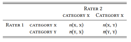
Table 4.3 shows a situation where the two raters assign one of the two categories x or y. Here, p_o would be the sum of n(x, x) and n(y, y), divided by the sum of all annotation; p_e can be calculated in various ways, a straightforward one will be introduced below.

Table 4.3: A contingency table for two raters and two categories

Let us look at a concrete case. In English, many semantic relations can be expressed by more than one linguistic structure. A prominent example is ‘possession’, which can be expressed in two main ways: either by the s -possessive (traditionally referred to as “genitive”) with the modifier marked by the clitic ’s (cf. 23a), or by the of -construction, with the modifier as a prepositional object of the preposition of (cf. 23b):

(23) a. a tired horse’s plodding step (BROWN K13)

b. every leaping stride of the horse (BROWN N02)

Let us assume that we want to investigate the factors determining the choice between these two constructions (as we will do in Chapters 5 and 6). In order to do so, we need to identify the subset of constructions with of that actually correspond to the s-possessive semantically – note that the of -construction encodes a wide range of relations, including many – for example quantification or partition – that are never expressed by an s -possessive. This means that we must manually go through the hits for the of -construction in our data and decide whether the relation encoded could also be encoded by an s -possessive. Let us use the term “of -possessive” for these cases. Ideally, we would do this by searching a large corpus for actual examples of paraphrases with the s -possessive, but let us assume that this is too time-consuming (a fair assumption in many research contexts) and that we want to rely on introspective judgments instead.

We might formulate a simple annotation scheme like the following:

For each case of the structure [(DET_i ) (AP_i ) N_i of NP_j ], paraphrase it as an s -possessive of the form [NP_j ’s (AP_i) N_i ] (for example, the leaping stride of the horse becomes the horse’s leaping stride). If the result sounds like something a speaker of English would use, assign the label POSS, if not, assign the label other.

In most cases, following this instruction should yield a fairly straightforward response, but there are more difficult cases. Consider (24a, b) and (25a, b), where the paraphrase sounds decidedly odd:

(24) a. a lack of unity

b. ^?? unity’s lack

(25) a. the concept of unity

b. ^?? unity’s concept

At first glance, neither of them seems to be paraphraseable, so they would both be assigned the value OTHER according to our annotation scheme. However, in a context that strongly favors s -possessives – namely, where the possessor is realized as a possessive determiner –, the paraphrase of (24a) sounds acceptable, while (25a) still sounds odd:

(26) a. Unity is important, and its lack can be a problem.

b. ^?? Unity is important, so its concept must be taught early.

Thus, we might want to expand our annotation scheme as follows:

For each case of the structure [(DET_i ) (AP_i ) N_i of NP_j ],

1. paraphrase it as an s -possessive of the form [NP_j ’s (AP_i ) N_i ] (for example, the leaping stride of the horse becomes the horse’s leaping stride). If the result sounds like something a speaker of English would use, assign the label POSS. If not,
2. replace NP_j by a possessive determiner (for example, the horse’s leaping stride becomes its leaping stride and construct a coordinated sentence with NPj as the subject of the first conjunct and [PDET_j (AP_i, ) N_i ] as the subject of the second conjunct (for example, The horse tired and its leaping stride shortened. If the s -possessive sounds like something a speaker of English would use in this context, assign the label poss,) if not, assign the label OTHER.

Obviously, it is no simple task to invent a meaningful context of the form required by these instructions and then deciding whether the result is acceptable. In other words, it is not obvious that this is a very reliable operationalization of the construct OF -POSSESSSIVE, and it would not be surprising if speakers’ introspective judgments varied too drastically to yield useful results.

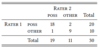
Table 4.4 shows a random sample of of -constructions from the BROWN corpus (with cases that have a quantifying noun like lot or bit instead of a regular noun as N_i already removed. The introspective judgments were derived by two different raters (both trained linguists who wish to remain anonymous) based on the instructions above. The tabulated data for both annotators are shown in Table 4.5.

As discussed above, the relative observed agreement is the percentage of cases both raters chose POSS or both raters chose OTHER, i.e.

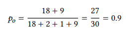
The relative expected agreement, i.e. the probability that both raters agree in their choice between POSS or OTHER by chance, can be determined as follows (we will return to this issue in the next chapter and keep it simple here). RATER 1 chose POSS with a probability of ²⁰/₃₀ = 0.6667 (i.e., 66.67 percent of the time) and OTHER with a probability of ¹⁰/₃₀ = 0.3333 (i.e., 33.33 percent of the time). RATER 2 chose POSS with a probability of ¹⁹/₃₀ = 0.6333, and OTHER with a probability of ¹¹/₃₀ = 0.3667.

The joint probability that both raters will choose poss by chance is the product of their individual probabilities of doing so, i.e. 0.6667 × 0.6333 = 0.4222; for no it is 0.3333 × 0.3667 = 0.1222. Adding these two probabilities gives us the overall probability that the raters will agree by chance: 0.4222 + 0.1222 = 0.5444.

Table 4.4: Paraphraseablility ratings for a sample of of -constructions by two raters

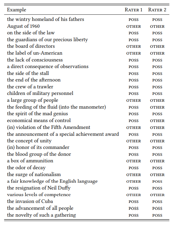
Table 4.5: Count of judgments from Table 4.4

We can now calculate the interrater reliability for the data in Table 4.4 using the formula in (22) above:

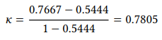
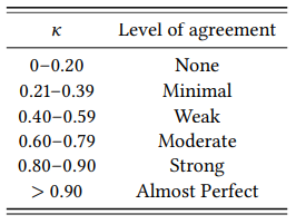
There are various suggestions as to what value of _K is to be taken as satisfactory. One reasonable suggestion (following McHugh 2012) is shown in Table 4.6; according to this table, our annotation scheme is good enough to achieve “strong” agreement between raters, and hence presumably good enough to use in a corpus linguistic research study (what is “good enough” obviously depends on the risk posed by cases where there is no agreement in classification).

Table 4.6: Interpretation of _K values

4.2.4 Reproducibility

Scientific research is collaborative and incremental in nature, with researchers building on and extending each other’s work. As discussed in the previous chapter in Section 3.3, this requires that we be transparent with respect to our data and methods to an extent that allows other researchers to reproduce our results. This is referred to as reproducibility and/or (with a different focus, replicability) – since there is some variation in how these terms are used, let us briefly switch to more specific, non-conventional terminology.

The minimal requirement of an incremental and collaborative research cycle is what we might call retraceability: our description of the research design and the associated procedures must be explicit and detailed enough for another researcher to retrace and check for correctness each step of our analysis and when provided with all our research materials (i.e., the corpora, the raw extracted data and the annotated data) and all other resources used (such as our annotation scheme and the software used in the extraction and statistical analysis of the data) and all our research notes, intermediate calculations, etc. In other words, our research project must be documented in sufficient detail for others to make sure that we arrived at our results via the procedures that we claim to have used, and to identify possible problems in our data and/or procedure. Thus retraceability is closely related to the idea of accountability in accounting.

Going slightly beyond retraceability, we can formulate a requirement which we might call reconstructibility: given all materials and resources, the description of our procedure must be detailed enough to ensure that a researcher independently applying this procedure to the same data using the same resources, but without access to our research notes, intermediate results, etc., should arrive at the same result.

Both of the requirements just described fall within the range of what is referred to as reproducibility. Obviously, as long as our data and other resources (and, if relevant, our research notes and intermediate results) are available, reproducibility is largely a matter of providing a sufficiently explicit and fine-grained description of the steps by which we arrived at our results. However, in actual practice it is surprisingly difficult to achieve reproducibility even if our research design does not involve any manual data extraction or annotation (see Stefanowitsch (2018) for an attempt). As soon as our design includes steps that involve manual extraction or annotation, it may still be retraceable, but it will no longer be reconstructible; however, if we ensure that our extraction methods and annotation scheme(s) have a high interrater reliability, an attempt at reconstruction should at least lead to very similar results.

Matters become even more difficult if our data or other resources are not accessible, for example, if we use a corpus or software constructed specifically for our research project that we cannot share publicly due to copyright restrictions, or if our corpus contains sensitive information such that sharing it would endanger individuals, violate non-disclosure agreements, constitute high treason, etc.

In such a case, our research will not be reproducible (retraceable or reconstructible), which is why we should avoid this situation. If it cannot be avoided, however, our research should still meet a requirement that we might call transferability: the description of our materials, resources and procedures must be detailed enough for other researchers to transfer it to similar materials and resources and arrive at a similar result. This is broadly what replicability refers to, but the term may also be used in an extended sense to situations where a researcher attempts to replicate our results and conclusions rather than our entire research design. Obviously, research designs that meet the criterion of reproducibility are also transferable, but not vice versa.

In the context of the scientific research cycle, reproducibility and replicability are crucial: a researcher building on previous research must be able to reconstruct this research in order to determine its quality and thus the extent to which our results can be taken to corroborate our hypotheses. They must also be able to reconstruct the research in order to build on it in a meaningful way, for example by adapting our methods to other kinds of data, new hypotheses or other linguistic phenomena.

Say, for example, a researcher wanted to extend the analysis of the words wind-screen and windshield presented in Chapter 3, Section 3.1 to other varieties of English. The first step would be to reconstruct our analysis (if they had access to the LOB, BROWN, FLOB and FROWN corpora), or to adapt it (for example, to the BNC and COCA, briefly mentioned at the end of our analysis). However, with the information provided in Chapter 3, this would be very difficult. First, there was no mention of which version of the LOB, BROWN, FLOB and FROWN was used (there are at least two official releases, one that was commercially available from an organization called ICAME and a different one that is available via the CLARIN network, and each of those releases contains different versions of each corpus). Second, there was no mention of the exact queries used – obviously, the words can be spelled in a range of ways, including at least WINDSCREEN, WIND SCREEN, WIND-SCREEN, Windscreen, Wind screen, Wind Screen, Wind-screen, Wind-Screen, windscreen, wind screen and wind-screen for WINDSCREEN, and the corresponding variants for WINDSHIELD. This range of graphemic variants can be searched for in different ways depending what annotation the respective version of the corpus contains, what software was used to access it and how we want to formulate our query. None of this information was provided in Chapter 3. Finally, nothing was said about how the total number of hits was calculated, which is not a problem in the case of a simple mathematical operation like addition, but which can quickly become relevant in the case of procedures and software used to evaluate the results statistically (as discussed in the next chapter).

It would not be surprising if a researcher attempting to reconstruct our analysis would get different results. This is not a purely theoretical possibility even with such a simple research design – you will often find that even word frequencies reported for a given corpus in the literature will not correspond to what your own query of the same corpus yields. Obviously, the more complex the phenomenon, the more difficult it will be to guess what query or queries a researcher has used if they do not tell us. And if the data had to be annotated in any way more complex than “number of letters”, that annotation will be difficult to reconstruct even if an annotation scheme is provided, and impossible to reconstruct if this is not the case.

Unfortunately, corpus linguists have long paid insufficient attention to this (and I include much of my own research in this criticism). It is high time that this change and that corpus linguists make an honest effort to describe their designs in sufficient detail to make them reproducible (in all senses discussed above). In many disciplines, it is becoming customary to provide raw data, categorized data, computer scripts, etc. in the form of supplementary materials with every research article. This is not yet standard in corpus linguistics, but it is a good idea to plan and document your research as though it already were.

4.2.5 Data storage

We will conclude this chapter with a discussion of a point that may, at first, appear merely practical but that is crucial in carrying out corpus-linguistic research (and that has some methodological repercussions, too): the question of how to store our data and annotation decisions. There are broadly two ways of doing so: first, in the corpus itself, and second, in a separate database of some sort.

The first option is routinely chosen in the case of automatically annotated variables like PART OF SPEECH, as in the passage from the BROWN corpus cited in Figure 2.4 in Chapter 2, repeated here partially as (27):

(27) the_AT fact_NN that_CS Jess's_NP$ horse_NN had_HVD not_*

been_BEN returned_VBN to_IN its_PP$ stall_NN could_MD

indicate_VB that_CS Diane's_NP$ information_NN had_HVD been_BEN wrong_JJ ,_, but_CC Curt_NP didn't_DOD* interpret_VB

it_PPO this_DT way_NN ._. (BROWN N12)

Here, the annotation (i.e., the part-of-speech tags) are attached to the data they refer to (i.e., words) by an underscore (recall that alternatively, a vertical format with words in the first and tags in the second column is frequently used, as are various kinds of XML notation).

The second option is more typically chosen in the case of annotations added in the context of a specific research project (especially if they are added manually): the data are extracted, stored in a separate file, and then annotated. Frequently, spreadsheet applications are used to store the corpus data and annotation decisions, as in the example in Figure 4.1, where possessive pronouns and nouns are annotated for NOMINAL TYPE, ANIMACY and CONCRETENESS:

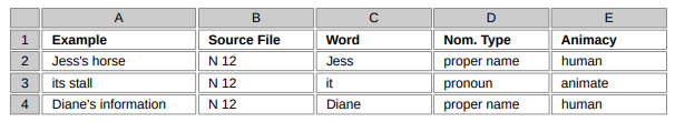
Figure 4.1: Example of a raw data table

The first line contains labels that tell us what information is found in each column respectively. This should include the example itself (either as shown in Figure 4.1, or in the form of a KWIC concordance line) and meta-information such as what corpus and/or corpus file the example was extracted from. Crucially, it will include the relevant variables. Each subsequent line contains one observation (i.e., one hit and the appropriate values of each variable). This format – one column for each variable, and one line for each example – is referred to as a raw data table. It is the standard way of recording measurements in all empirical sciences and we should adhere to it strictly, as it ensures that the structure of the data is retained.

In particular, we should never store our data in summarized form, for example, as shown in Figure 4.2.

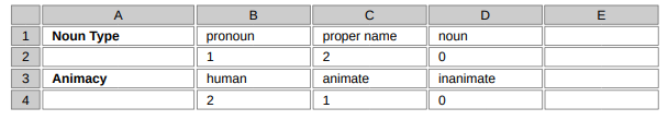
Figure 4.2: Data stored in summarized form

There is simply no need to store data in this form – if we need this kind of summary, it can be created automatically from a raw data table like that in Figure 4.1 – all major spreadsheet applications and statistical software packages have this functionality. What is more, statistics software packages require a raw data table of the kind shown in Figure 4.1 as input for most kinds of statistical analysis.

As mentioned above, however, the format of storage is not simply a practical matter, but a methodological one. If we did store our data in the form shown in Figure 4.2 straight away, we would irreversibly destroy the relationship between the corpus hits and the different annotations applied to them. In other words, we would have no way of telling which combinations of variables actually occurred in the data. In Figure 4.2, for example, we cannot tell whether the pronoun referred to one one of the human referents or to the animate referent. Even if we do not need to know these relationships in the context of a given research project (or initially believe we will not), we should avoid this situation, as we do not know what additional questions may come up in the course of our research that do require this information.

Since quantitative analysis always requires a raw data table, we might conclude that it is the only useful way of recording our annotation decisions. However, there are cases where it may be more useful to record them in the form of annotations in (a copy of) the original corpus instead, i.e., analogously to automatically added annotations. For example, the information in Figure 4.1 could be recorded in the corpus itself in the same way that part-of-speech tags are, i.e., we could add an ANIMACY label to every nominal element in our corpus in the format used for POS tags by the original version of the BROWN corpus, as shown in (28):

(28) the_AT fact_NN_abstract that_CS Jess's_NP$_human horse_NN_animate had_HVD not_* been_BEN returned_VBN to_IN its_PP$_animate stall_NN_inanimate could_MD indicate_VB that_CS Diane's_NP$_human information_NN_abstract had_HVD been_BEN wrong_JJ ,_, but_CC Curt_NP_human didn't_DOD* interpret_VB it_PPO_inanimate this_DT way_NN_inanimate ._.

From a corpus annotated in this way, we can always create a raw data list like that in Figure 4.1 by searching for possessives and then separating the hits into the word itself, the PART-OF-SPEECH label and the ANIMACY annotation (this can be done manually, or with the help of regular expressions in a text editor or with a few lines of code in a scripting language like Perl or Python).

The advantage would be that we, or other researchers, could also use our annotated data for research projects concerned with completely different research questions. Thus, if we are dealing with a variable that is likely to be of general interest, we should consider the possibility of annotating the corpus itself, instead of first extracting the relevant data to a raw data table and annotating them afterwards. While the direct annotation of corpus files is rare in corpus linguistics, it has become the preferred strategy in various fields concerned with qualitative analysis of textual data. There are open-source and commercial software packages dedicated to this task. They typically allow the user to define a set of annotation categories with appropriate codes, import a text file, and then assign the codes to a word or larger textual unit by selecting it with the mouse and then clicking a button for the appropriate code that is then added (often in XML format) to the imported text. This strategy has the additional advantage that one can view one’s annotated examples in their original context (which may be necessary when annotating additional variables later). However, the available software packages are geared towards the analysis of individual texts and do not let the user to work comfortably with large corpora.

³ In fact, it may be worth exploring, within a corpus-linguistic framework, ways of annotating data that are based entirely on implicit decisions by untrained speakers; specifically, I am thinking here of the kinds of association tasks and sorting tasks often used in psycholinguistic studies of word meaning.

⁴ For more than two raters, there is a more general version of this metric, referred to as Fleiss’ _K (Fleiss 1971), but as it is typically difficult even to find a second annotator, we will stick with the simpler measure here.