9.1: Quantifying morphological phenomena

9.1.1 Counting morphemes: Types, tokens and hapax legomena

Determining the frequency of a linguistic phenomenon in a corpus or under a particular condition seems a straightforward task: we simply count the number of instances of this phenomenon in the corpus or under that condition. However, this sounds straightforward (in fact, tautological) only because we have made tacit assumptions about what it means to be an “instance” of a particular phenomenon.

When we are interested in the frequency of occurrence of a particular word, it seems obvious that every occurrence of the word counts as an instance. In other words, if we know how often the word occurs in our data, we know how many instances there are in our data. For example, in order to determine the number of instances of the definite article in the BNC, we construct a query that will retrieve the string the in all combinations of upper and lower case letters, i.e. at least the, The, and THE, but perhaps also tHe, ThE, THe, tHE and thE, just to be sure). We then count the hits (since this string corresponds uniquely to the word the, we don’t even have to clean up the results manually). The query will yield 6 041 234 hits, so there are 6 041 234 instances of the word the in the BNC.

When searching for grammatical structures (for example in Chapters 5 and 6), simply transferred this way of counting occurrences. For example, in order to determine the frequency of the s-possessive in the BNC, we would define a reasonable query or set of queries (which, as discussed in various places in this book, can be tricky) and again simply count the hits. Let us assume that the query \(\langle\text{[pos="(POS|DPS)"] [pos=".*AJ.*"]? [pos=".*NN.*"]}\rangle\) is a reasonable approximation: it retrieves all instances of the possessive clitic (tagged \(\text{POS}\) in the BNC) or a possessive determiner (\(\text{DPS}\)), optionally followed by a word tagged as an adjective (\(\text{AJ0}\), \(\text{AJC}\) or \(\text{AJS}\), even if it is part of an ambiguity tag), followed by a word tagged as a noun (\(\text{NN0}\), \(\text{NN1}\) or \(\text{NN2}\), even if it is part of an ambiguity tag). This cquery will retrieve 1 651 908 hits, so it seems that there are 1 651 908 instances of the s-possessive in the BNC.

However, there is a crucial difference between the two situations: in the case of the word the, every instance is identical to all others (if we ignore upper and lower case). This is not the case for the s-possessive. Of course, here, too, many instances are identical to other instances: there are exact repetitions of proper names, like King’s Cross (322 hits) or People’s revolutionary party (47), of (parts of) idiomatic expressions, like arm’s length (216) or heaven’s sake (187) or non-idiomatic but nevertheless fixed phrases like its present form (107) or child’s best interest (26), and also of many free combinations of words that recur because they are simply communicatively useful in many situations, like her head (5105), his younger brother (112), people’s lives (224) and body’s immune system (29).

This means that there are two different ways to count occurrences of the s-possessive. First, we could simply count all instances without paying any attention to whether they recur in identical form or not. When looking at occurrences of a linguistic item or structure in this way, they are referred to as tokens, so 1 651 908 is the token frequency of the possessive. Second, we could exclude repetitions and count only the number of instances that are different from each other, for example, we would count King’s Cross only the first time we encounter it, disregarding the other 321 occurrences. When looking at occurrences of linguistic items in this way, they are referred to as types; the type frequency of the s-possessive in the BNC is 268 450 (again, ignoring upper and lower case). The type frequency of the, of course, is 1.

Let us look at one more example of the type/token distinction before we move on. Consider the following famous line from the theme song of the classic television series “Mister Ed”:

1. A horse is a horse, of course, of course...

At the word level, it consists of nine tokens (if we ignore punctuation): a, horse, is, a, horse, of, course, of, and course, but only of five types: a, horse, is, of, and course. Four of these types occur twice, one (is) occurs only once. At the level of phrase structure, it consists of seven tokens: the NPs a horse, a horse, course, and course, the PPs of course and of course, and the VP is a horse, but only of three types: VP, NP and PP.

In other words, we can count instances at the level of types or at the level of tokens. Which of the two levels is relevant in the context of a particular research design depends both on the kind of phenomenon we are counting and on our research question. When studying words, we will normally be interested in how often they are used under a particular condition, so it is their token frequency that is relevant to us; but we could imagine designs where we are mainly interested in whether a word occurs at all, in which case all that is relevant is whether its type frequency is one or zero. When studying grammatical structures, we will also mainly be interested in how frequently a particular grammatical structure is used under a certain condition, regardless of the words that fill this structure. Again, it is the token frequency that is relevant to us. However, note that we can (to some extent) ignore the specific words filling our structure only because we are assuming that the structure and the words are, in some meaningful sense, independent of each other; i.e., that the same words could have been used in a different structure (say, an of -possessive instead of an s-possessive) or that the same structure could have been used with different words (e.g. John’s spouse instead of his wife). Recall that in our case studies in Chapter 6 we excluded all instances where this assumption does not hold (such as proper names and fixed expressions); since there is no (or very little) choice with these cases, including them, let alone counting repeated occurrences of them, would have added nothing (we did, of course, include repetitions of free combinations, of which there were four in our sample: his staff, his mouth, his work and his head occurred twice each).

Obviously, instances of morphemes (whether inflectional or derivational) can be counted in the same two ways. Take the following passage from William Shakespeare’s play Julius Cesar:

2. CINNA: ... Am I a married man, or a bachelor? Then, to answer every man directly and briefly, wisely and truly: wisely I say, I am a bachelor.

Let us count the occurrences of the adverbial suffix -ly. There are five word tokens that contain this suffix (directly, briefly, wisely, truly, and wisely), so its token frequency is five; however, there are only four types, since wisely occurs twice, so its type frequency in this passage is four.

Again, whether type or token frequency is the more relevant or useful measure depends on the research design, but the issue is more complicated than in the case of words and grammatical structures. Let us begin to address this problem by looking at the diminutive affixes -icle (as in cubicle, icicle) and mini- (as in minivan, mini-cassette).

9.1.1.1 Token frequency

First, let us count the tokens of both affixes in the BNC. This is relatively easy in the case of -icle, since the string \(\text{icle}\) is relatively unique to this morpheme (the name Pericles is one of the few false hits that the query \(\langle\text{[word=".+icles?"%c]}\rangle\) will retrieve). It is more difficult in the case of mini-, since there are words like minimal, minister, ministry, miniature and others that start with the string \(\text{mini}\) but do not contain the prefix mini-. Once we have cleaned up our concordances (available in the Supplementary Online Material, file LMY7), we will find that -icle has a token frequency of 20 772 – more than ten times that of mini-, which occurs only 1702 times. We might thus be tempted to conclude that -icle is much more important in the English language than mini-, and that, if we are interested in English diminutives, we should focus on -icle. However, this conclusion would be misleading, or at least premature, for reasons related to the problems introduced above.

Recall that affixes do not occur by themselves, but always as parts of words (this is what makes them affixes in the first place). This means that their token frequency can reflect situations that are both quantitatively and qualitatively very different. Specifically, a high token frequency of an affix may be due to the fact that it is used in a small number of very frequent words, or in a large number of very infrequent words (or something in between). The first case holds for -icle: the three most frequent words it occurs in (article, vehicle and particle) account for 19 195 hits (i.e., 92.41 percent of all occurrences). In contrast, the three most frequent words with mini- (mini-bus, mini-bar and mini-computer) account for only 557 hits, i.e. 32.73 percent of all occurrences. To get to 92.4 percent, we would have to include the 253 most frequent words (roughly two thirds of all types).

In other words, the high token frequency of -icle tells us nothing (or at least very little) about the importance of the affix; if anything, it tells us something about the importance of some of the words containing it. This is true regardless of whether we look at its token frequency in the corpus as a whole or under specific conditions; if its token frequency turned out to be higher under one condition than under the other, this would point to the association between that condition and one or more of the words containing the affix, rather than between the condition and the affix itself.

For example, the token frequency of the suffix -icle is higher in the BROWN corpus (269 tokens) than in the LOB corpus (225 tokens). However, as \(Table \text{ } 9.1\) shows, this is simply due to differences in the frequency of individual words – the words particle and vehicle are substantially more frequent in the BROWN corpus, and while, conversely, article is more frequent in the LOB corpus, it cannot make up for the difference. As the \(\chi^{2}\) components show, the difference in frequency of some of the individual words is even statistically significant, but nothing follows from this with respect to the suffix -icle.

\(Table \text { } 9.1\): Words containing -icle in two corpora

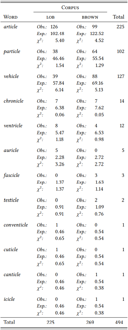
Even if all words containing a particular affix were more frequent under one condition (e.g. in one variety) than under another, this would tell us nothing certain about the affix itself: while such a difference in frequency could be due to the affix itself (as in the case of the adverbial suffix -ly, which is disappearing from American English, but not from British English), it could also be due exclusively to the words containing the affix.

This is not to say that the token frequencies of affixes can never play a useful role; they may be of interest, for example, in cases of morphological alternation (i.e. two suffixes competing for the same stems, such as -ic and -ical in words like electric/al); here, we may be interested in the quantitative association between particular stems and one or the other of the affix variants, essentially giving us a collocation-like research design based on token frequencies. But for most research questions, the distribution of token frequencies under different conditions is meaningless.

9.1.1.2 Type frequency

In contrast, the type frequency of an affix is a fairly direct reflection of the importance of the affix for the lexicon of a language: obviously an affix that occurs in many different words is more important than one that occurs only in a few words. Note that in order to compare type frequencies, we have to correct for the size of the sample: all else being equal, a larger sample will contain more types than a smaller one simply because it offers more opportunities for different types to occur (a point we will return to in more detail in the next subsection). A simple way of doing this is to divide the number of types by the number of tokens; the resulting measure is referred to very transparently as the type/token ratio (or TTR):

3. \(\mathrm{TTR}=\frac{n(\text { types })}{n(\text { tokens })}\)

The TTR is the percentage of types in a sample are different from each other; or, put differently, it is the mean probability that we will encounter a new type if we go through the sample item by item.

For example, the affix -icle occurs in just 31 different words in the BNC, so its TTR is \(\frac{31}{20772}\) = 0.0015. In other words, 0.15 percent of its tokens in the BNC are different from each other, the vast remainder consists of repetitions. Put differently, if we go through the occurrences of -icle in the BNC item by item, the probability that the next item instantiating this suffix will be a type we have not seen before is 0.15 percent, so we will encounter a new type on average once every 670 words. For mini-, the type-token ratio is much higher: it occurs in 382 different words, so its TTR is \(\frac{382}{1702}\) = 0.2244. In other words, almost a quarter of all occurrences of mini- are different from each other. Put differently, if we go through the occurrences of mini- in the BNC word by word, the probability that the next instance is a new type would be 22.4 percent, so we will encounter a new type about every four to five hits. The differences in their TTRs suggests that mini-, in its own right, is much more central in the English lexicon than -icle, even though the latter has a much higher token frequency. Note that this is a statement only about the affixes; it does not mean that the words containing mini- are individually or collectively more important than those containing -icle (on the contrary: words like vehicle, article and particle are arguably much more important than words like minibus, minicomputer and minibar).

Likewise, observing the type frequency (i.e. the TTR) of an affix under different conditions provides information about the relationship between these conditions and the affix itself, albeit one that is mediated by the lexicon: it tells us how important the suffix in question is for the subparts of the lexicon that are relevant under those conditions. For example, there are 7 types and 9 tokens for mini- in the 1991 British FLOB corpus (two tokens each for mini-bus and mini-series and one each for mini-charter, mini-disc, mini-maestro, mini-roll and mini-submarine), so the TTR is \(\frac{7}{9}\) = 0.7779. In contrast, in the 1991 US-American FROWN corpus, there are 11 types and 12 tokens (two tokens for mini-jack, and one token each for mini-cavalry, mini-cooper, mini-major, mini-retrospective, mini-version, mini-boom, mini-camp, mini-grinder, mini-series, and mini-skirt), so the TTR is \(\frac{11}{12}\) = 0.9167. This suggests that the prefix mini- was more important to the US-English lexicon than to the British English lexicon in the 1990s, although, of course, the samples and the difference between them are both rather small, so we would not want to draw that conclusion without consulting larger corpora and, possibly, testing for significance first (a point I will return to in the next subsection).

9.1.1.3 Hapax legomena

While type frequency is a useful way of measuring the importance of affixes in general or under specific conditions, it has one drawback: it does not tell us whether the affix plays a productive role in a language at the time from which we take our samples (i.e. whether speakers at that time made use of it when coining new words). An affix may have a high TTR because it was productively used at the time of the sample, or because it was productively used at some earlier period in the history of the language in question. In fact, an affix can have a high TTR even if it was never productively used, for example, because speakers at some point borrowed a large number of words containing it; this is the case for a number of Romance affixes in English, occurring in words borrowed from Norman French but never (or very rarely) used to coin new words. An example is the suffix -ence/-ance occurring in many Latin and French loanwords (such as appearance, difference, existence, influence, nuisance, providence, resistance, significance, vigilance, etc.), but only in a handful of words formed in English (e.g. abidance, forbearance, furtherance, hinderance, and riddance).

In order to determine the productivity (and thus the current importance) of affixes at a particular point in time, Harald Baayen (cf. e.g. Baayen 2009 for an overview) has suggested that we should focus on types that only occur once in the corpus, so-called hapax legomena (Greek for ‘said once’). The assumption is that productive uses of an affix (or other linguistic rule) should result in one-off coinages (some of which may subsequently spread through the speech community while others will not).

Of course, not all hapax legomena are the result of productive rule-application: the words wordform-centeredness and ingenuity that I used in the first sentence of this chapter are both hapax legomena in this book (or would be, if I did not keep mentioning them). However, wordform-centeredness is a word I coined productively and which is (at the time of writing) not documented anywhere outside of this book; in fact, the sole reason I coined it was in order to use it as an example of a hapax legomenon later). In contrast, ingenuity has been part of the English language for more than four-hundred years (the OED first records it in 1598); it occurs only once in this book for the simple reason that I only needed it once (or pretended to need it, to have another example of a hapax legomenon). So a word may be a hapax legomenon because it is a productive coinage, or because it is infrequently needed (in larger corpora, the category of hapaxes typically also contains misspelled or incorrectly tokenized words which will have to be cleaned up manualy – for example, the token manualy is a hapax legomenon in this book because I just misspelled it intentionally, but the word manually occurs dozens of times in this book).

Baayen’s idea is quite straightforwardly to use the phenomenon of hapax legomenon as an operationalization of the construct “productive application of a rule” in the hope that the correlation between the two notions (in a large enough corpus) will be substantial enough for this operationalization to make sense.¹

Like the number of types, the number of hapax legomena is dependent on sample size (although the relationship is not as straightforward as in the case of types, see next subsection); it is useful, therefore, to divide the number of hapax legomena by the number of tokens to correct for sample size:

4. \(\mathrm{HTR}=\frac{n(\text { hapax legomena })}{n(\text { tokens })}\)

We will refer to this measure as the hapax-token ratio (or HTR) by analogy with the term type-token ratio. Note, however, that in the literature this measure is referred to as P for “Productivity” (following Baayen, who first suggested the measure); I depart from this nomenclature here to avoid confusion with p for “probability (of error)”.

Let us apply this measure to our two diminutive affixes. The suffix -icle has just five hapax legomena in the BNC (auricle, denticle, pedicle, pellicle and tunicle). This means that its HTR is \(\frac{5}{20772}\) = 0.0002, so 0.02 percent of its tokens are hapax legomena. In contrast, there are 247 hapax legomena for mini- in the BNC (including, for example, mini-earthquake, mini-daffodil, mini-gasometer, mini-cow and mini-wurlitzer). This means that its HTR is \(\frac{247}{1702}\) = 0.1451, so 14.5 percent of its tokens are hapax legomena. Thus, we can assume that mini- is much more productive than -icle, which presumably matches the intuition of most speakers of English.

9.1.2 Statistical evaluation

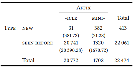
As pointed out in connection with the comparison of the TTRs for mini- in the FLOB and the FROWN corpus, we would like to be able to test differences between two (or more) TTRs (and, of course, also two or more HTRs) for statistical significance. Theoretically, this could be done very easily. Take the TTR: if we interpret it as the probability of encountering a new type as we move through our samples, we are treating it like a nominal variable \(\text{Type}\), with the values \(\text{new}\) and \(\text{seen before}\). One appropriate statistical test for distributions of nominal values under different conditions is the \(\chi^{2}\) test, which we are already more than familiar with. For example, if we wanted to test whether the TTRs of -icle and mini- in the BNC differ significantly, we might construct a table like \(Table \text { } 9.2\).

The \(\chi^{2}\) test would tell us that the difference is highly significant with a respectable effect size (\(\chi^{2}\) = 4334.67, df = 1, \(p\) < 0.001, \(\phi\) = 0.4392). For HTRs, we could follow a similar procedure: in this case we are dealing with a nominal variable \(\text{Type}\) with the variables \(\text{occurs only once}\) and \(\text{occurs more than once}\), so we could construct the corresponding table and perform the \(\chi^{2}\) test.

\(Table \text { } 9.2\): Type/token ratios of -icle and mini- in the BNC

However, while the logic behind this procedure may seem plausible in theory both for HTRs and for TTRs, in practice, matters are much more complicated. The reason for this is that, as mentioned above, type-token ratios and hapax-token ratios are dependent on sample size.

In order to understand why and how this is the case and how to deal with it, let us leave the domain of morphology for a moment and look at the relationship between tokens and types or hapax legomena in texts. Consider the opening sentences of Jane Austen’s novel Pride and Prejudice (the novel is freely available from Project Gutenberg and in the Supplementary Online Material, file TXQP):

5. It is a truth universally acknowledged, that a_2/-1 single man in possession of a₃ good fortune, must be in_2/-1 want of_2/-1 a₄ wife. However little known the feelings or views of₃ such a₅ man_2/-1 may be_2/-1 on his first entering a₆ neighbourhood, this truth_2/-1 is_2/-1 so well fixed in₃ the_2/-1 minds of₄ the surrounding families, that_2/-1 he is₃ considered the rightful property of₅ some one or_2/-1 other of₆ their daughters.

All words without a subscript are new types and hapax legomena at the point at which they appear in the text; if a word has a subscript, it means that it is a repetition of a previously mentioned word, the subscript is its token frequency at this point in the text. The first repetition of a word is additionally marked by a subscript reading -1, indicating that it ceases to be hapax legomenon at this point, decreasing the overall count of hapaxes by one.

As we move through the text word by word, initially all words are new types and hapaxes, so the type- and hapax-counts rise at the same rate as the token counts. However, it only takes eight token before we reach the first repetition (the word a), so while the token frequency rises to 8, the type count remains constant at seven and the hapax count falls to six. Six words later, there is another occurrence of a, so type and hapax counts remain, respectively, at 12 and 11 as the token count rises to 14, and so on. In other words, while the number of types and the number of hapaxes generally increase as the number of tokens in a sample increases, they do not increase at a steady rate. The more types have already occurred, the more types there are to be reused (put simply, speakers will encounter fewer and fewer communicative situations that require a new type), which makes it less and less probable that new types (including new hapaxes) will occur. \(Figure \text { } 9.1\) shows how type and hapax counts develop in the first 100 words of Pride and Prejudice (on the left) and in the whole novel (on the right).

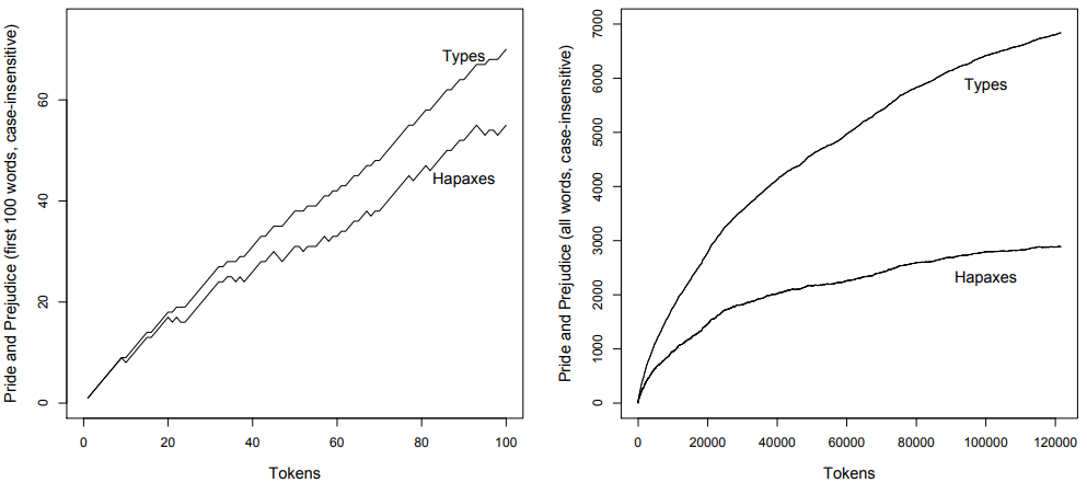
\(Figure \text { } 9.1\): TTR and HTR in Jane Austen’s Pride and Prejudice

As we can see by looking at the first 100 words, type and hapax counts fall below the token counts fairly quickly: after 20 tokens, the TTR is \(\frac{18}{20}\) = 0.9 and the HTR is \(\frac{17}{20}\) = 0.85, after 40 tokens the TTR is \(\frac{31}{40}\) = 0.775 and the HTR is \(\frac{26}{40}\) = 0.65, after 60 tokens the HTR is \(\frac{42}{60}\) = 0.7 and the TTR is \(\frac{33}{60}\) = 0.55, and so on (note also how the hapax-token ratio sometimes drops before it rises again, as words that were hapaxes up to a particular point in the text reoccur and cease to be counted as hapaxes). If we zoom out and look at the entire novel, we see that the growth in hapaxes slows considerably, to the extent that it has almost stopped by the time we reach the end of the novel. The growth in types also slows, although not as much as in the case of the hapaxes. In both cases this means that the ratios will continue to fall as the number of tokens increases.

Now imagine we wanted to use the TTR and the HTR as measures of Jane Austen’s overall lexical productivity (referred to as “lexical richness” in computational stylistics and in second-language teaching): if we chose a small sample of her writing, the TTR and the HTR would be larger than if we chose a large sample, to the extent that the scores derived from the two samples would differ significantly. \(Table \text { } 9.3\) shows what would happen if we compared the TTR of the first chapter with the TTR of the entire rest of the novel.

\(Table \text { } 9.3\): Type/token ratios in the novel Pride and Prejudice

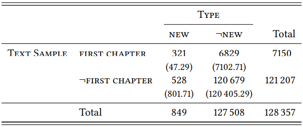
The TTR for the first chapter is an impressive 0.3781, that for the rest of the novel is a measly 0.0566, and the difference is highly significant (\(\chi^{2}\) = 1688.7, df = 1, \(p\) < 0.001, \(\phi\) = 0.1147). But this is not because there is anything special about the first chapter; the TTR for the second chapter is 0.3910, that for the third is 0.3457, that for chapter 4 is 0.3943, and so on. The reason why the first chapter (or any chapter) looks as though it has a significantly higher TTR than the novel as a whole is simply because the TTR will drop as the size of the text increases.

Therefore, comparing TTRs derived from samples of different sizes will always make the smaller sample look more productive. In other words, we cannot compare such TTRs, let alone evaluate the differences statistically – the result will simply be meaningless. The same is true for HTRs, with the added problem that, under certain circumstances, it will decrease at some point as we keep increasing the sample size: at some point, all possible words will have been used, so unless new words are added to the language, the number of hapaxes will shrink again and finally drop to zero when all existing types have been used at least twice.

We will encounter the same problem when we compare the TTR or HTR of particular affixes or other linguistic phenomena, rather than that of a text. Consider \(Figures \text { } 9.2a\) and \(9.2b\), which show the TTR and the HTR of the verb suffixes -ise/-ize (occurring in words like realize, maximize or liquidize) and -ify (occurring in words like identify, intensify or liquify).

As we can see, the TTR and HTR of both affixes behave roughly like that of Jane Austen’s vocabulary as a whole as we increase sample size: both of them

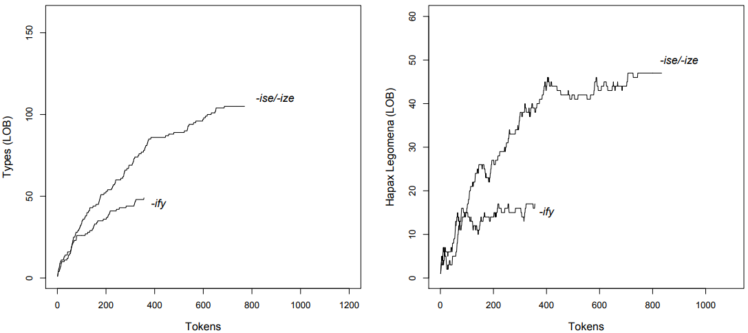
\(Figure \text { } 9.2\): (a) TTRs and (b) HTRs for -ise/-ize and -ify in the LOB corpus

grow fairly quickly at first before their growth slows down; the latter happens more quickly in the case of the HTR than in the case of the TTR, and, again, we observe that the HTR sometimes decreases as types that were hapaxes up to a particular point in the sample reoccur and cease to be hapaxes.

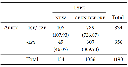
Taking into account the entire sample, the TTR for -ise/-ize is \(\frac{105}{834}\) = 0.1259 and that for -ify is \(\frac{49}{356}\) = 0.1376; it seems that -ise/-ize is slightly more important to the lexicon of English than -ify. A \(\chi^{2}\) test suggests that the difference is not significant (cf. \(Table \text { } 9.4\); \(\chi^{2}\) = 0.3053, df = 1, \(p\) > 0.05).

\(Table \text { } 9.4\): Type/token ratios of -ise/-ize and -ify (LOB)

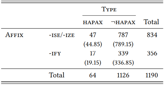
Likewise, taking into account the entire sample, the HTR for -ise/-ize is \(\frac{47}{834}\) = 0.0563 and that for -ify is \(\frac{17}{365}\) = 0.0477; it seems that -ise/-ize is slightly more productive than -ify. However, again, the difference is not significant (cf. \(Table \text { } 9.5\); \(\chi^{2}\) = 0.3628, df = 1, \(p\) > 0.05).

\(Table \text { } 9.5\): Hapax/token ratios of -ise/-ize and -ify (LOB)

However, note that -ify has a token frequency that is less than half of that of -ise/-ize, so the sample is much smaller: as in the example of lexical richness in Pride and Prejudice, this means that the TTR and the HTR of this smaller sample are exaggerated and our comparisons in \(Tables \text { } 9.4\) and \(9.5\) as well as the accompanying statistics are, in fact, completely meaningless.

The simplest way of solving the problem of different sample sizes is to create samples of equal size for the purposes of comparison. We simply take the size of the smaller of our two samples and draw a random sample of the same size from the larger of the two samples (if our data sets are large enough, it would be even better to draw random samples for both affixes). This means that we lose some data, but there is nothing we can do about this (note that we can still include the discarded data in a qualitative description of the affix in question).²

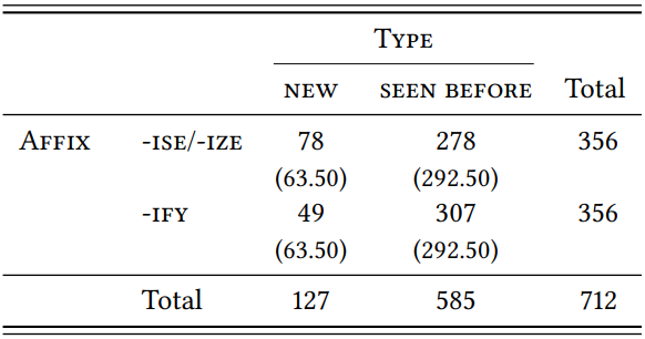
\(Figures \text { } 9.3a\) and \(9.3b\) show the growth rates of the TTR and the HTR of a subsample of 356 tokens of -ise/-ize in comparison with the total sample of the same size for -ify (the sample was derived by first deleting every second hit, then every seventh hit and finally every ninetieth hit, making sure that the remaining hits are spread throughout the corpus).

The TTR of -ise/-ize based on the random sub-sample is \(\frac{78}{356}\) = 0.2191, that of -ify is still \(\frac{49}{356}\) = 0.1376; the difference between the two suffixes is much clearer now, and a \(\chi^{2}\) test shows that it is very significant, although the effect size is weak (cf. \(Table \text { } 9.6\); \(\chi^{2}\) = 8.06, df = 1, \(p\) < 0.01, \(\phi\) = 0.1064).

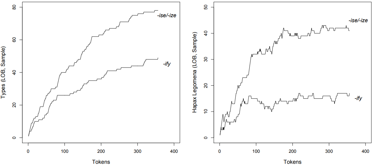
\(Figure \text { } 9.3\): (a) TTRs and (b) HTRs for -ise/-ize and -ify in the LOB corpus

\(Table \text { } 9.6\): Type/token ratios of -ise/-ize/-ise/-ize (sample) and -ify (LOB)

\(Table \text { } 9.7\): Hapax/token ratios of -ise/-ize (sample) and -ify (LOB)

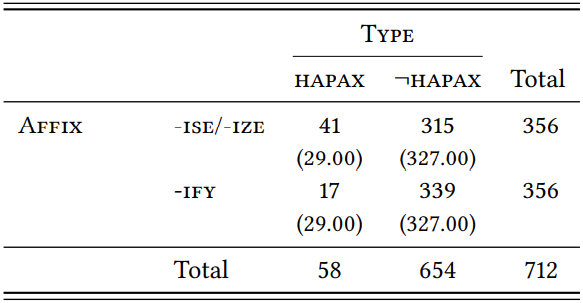
Likewise, the HTR of -ise/-ize based on our sub-sample is \(\frac{41}{356}\) = 0.1152, the HTR of -ify remains \(\frac{17}{365}\) = 0.0477. Again, the difference is much clearer, and it, too, is now very significant, again with a weak effect size (cf. \(Table \text { } 9.7\); \(\chi^{2}\) = 10.81, df = 1, \(p\) < 0.01, \(\phi\) = 0.1232).

In the case of the HTR, decreasing the sample size is slightly more problematic than in the case of the TTR. The proportion of hapax legomena actually resulting from productive rule application becomes smaller as sample size decreases. Take example (2) from Shakespeare’s Julius Caesar above: the words directly, briefly and truly are all hapaxes in the passage cited, but they are clearly not the result of a productively applied rule-application (all of them have their own entries in the OALD, for example). As we increase the sample, they cease to be hapaxes (directly occurs 9 times in the entire play, briefly occurs 4 times and truly 8 times). This means that while we must draw random samples of equal size in order to compare HTRs, we should make sure that these samples are as large as possible.

___________________________

¹Note also that the productive application of a suffix does not necessarily result in a hapax legomenon: two or more speakers may arrive at the same coinage, or a single speaker may like their own coinage so much that they use it again; some researchers therefore suggest that we should also pay attention to “dis legomena” (words occurring twice) or even “tris legomena” (words occurring three times). We will stick with the mainstream here and use only hapax legomena.
²In studies of lexical richness, a measure called Mean Segmental Type-Token Ratio (MSTTR) is sometimes used (cf. Johnson 1944). This measure is derived by dividing the texts under investigation into segments of equal size (often segments of 100 words), determining the TTR for each segment, and then calculating an average TTR. This allows us to compare the TTR of texts of different sizes without discarding any data. However, this method is not applicable to the investigation of morphological productivity, as most samples of 100 words (or even 1000 or 10 000 words) will typically not contain enough cases of a given morpheme to determine a meaningful TTR.