9.2: Case studies

9.2.1 Morphemes and stems

One general question in (derivational) morphology concerns the category of the stem which an affix may be attached to. This is obviously a descriptive issue that can be investigated on the basis of corpora very straightforwardly simply by identifying all types containing the affix in question and describing their internal structure. In the case of affixes with low productivity, this will typically add little insight over studies based on dictionaries, but for productive affixes, a corpus analysis will yield more detailed and comprehensive results since corpora will contain spontaneously produced or at least recently created items not (yet) found in dictionaries. Such newly created words will often offer particularly clear insights into constraints that an affix places on its stems. Finally, corpus-based approaches are without an alternative in diachronic studies and yield particularly interesting results when used to study changes in the quality or degree of productivity, (cf. for example Dalton-Puffer 1996).

In the study of constraints placed by derivational affixes on the stems that they combine with, the combinability of derivational morphemes (in an absolute sense or in terms of preferences) is of particular interest.Again, corpus linguistics is a uniquely useful tool to investigate this.

Finally, there are cases where two derivational morphemes are in direct competition because they are functionally roughly equivalent (e.g. -ness and -ity, both of which form abstract nouns from typically adjectival bases, -ise/-ize and -ify, which form process verbs from nominal and adjectival bases, or -ic and -ical, which form adjectives from typically nominal bases). Here, too, corpus linguistics provides useful tools, for example to determine whether the choice between affixes is influenced by syntactic, semantic or phonological properties of stems.

9.2.1.1 Case study: Phonological constraints on -ify

As part of a larger argument that -ise/-ize and -ify should be considered phonologically conditioned allomorphs, Plag (1999) investigates the phonological constraints that -ify places on its stems. First, he summarizes the properties of stems in established words with -ify as observed in the literature. Second, he checks these observations against a sample of twenty-three recent (20th century) coinages from a corpus of neologisms to ensure that the constraints also apply to productive uses of the affix. This is a reasonable approach. The affix was first borrowed into English as part of a large number of French loanwords beginning in the late 13th century; two thirds of all non-hapax types and 19 of the 20 most frequent types found in the BNC are older than the 19th century. Thus, it is possible that the constraints observed in the literature are historical remnants not relevant to new coinages.

The most obvious constraint is that the syllable directly preceding -ify must carry the main stress of the word. This has a number of consequences, of which we will focus on two: First, monosyllabic stems (as in falsify) are preferred, since they always meet this criterion. Second, if a polysyllabic stem ends in an unstressed syllable, the stress must be shifted to that syllable (as in perSONify from PERson);³ since this reduces the transparency of the stem, there should be a preference for those polysyllabic stems which already have the stress on the final syllable.

Plag simply checks his neologisms against the literature, but we will evaluate the claims from the literature quantitatively. Our main hypothesis will be that neologisms with -ify do not differ from established types with respect to the fact that the syllable directly preceding the suffix must carry primary stress, with the consequences that (i) they prefer monosyllabic stems, and (ii) if the stem is polysyllabic, they prefer stems that already have the primary stress on the last syllable. Our independent variable is therefore \(\mathrm{Lexical \space Status}\) with the values \(\mathrm{established \space word \space vs. \space neologism}\) (which will be operationalized presently). Our dependent variables are \(\mathrm{Syllabicity}\) with the values \(\mathrm{monosyllabic}\) and \(\mathrm{polysyllabic}\), and \(\mathrm{Stress \space Shift}\) with the values \(\mathrm{required \space vs. \space not \space required}\) (both of which should be self-explanatory).

Our design compares two predefined groups of types with respect to the distribution that particular properties have in these groups; this means that we do not need to calculate TTRs or HTRs, but that we need operational definitions of the values \(\mathrm{established \space word}\) and \(\mathrm{neologism}\). Following Plag, let us define \(\mathrm{neologism}\) as “coined in the 20th century”, but let us use a large historical dictionary (the Oxford English Dictionary, 3rd edition) and a large corpus (the BNC) in order to identify words matching this definition; this will give us the opportunity to evaluate the idea that hapax legomena are a good way of operationalizing productivity.

Excluding cases with prefixed stems, the OED contains 456 entries or sub-entries for verbs with -ify, 31 of which are first documented in the 20th century. Of the latter, 21 do not occur in the BNC at all, and 10 do occur in the BNC, but are not hapaxes (see \(Table \text { } 9.8\) below). The BNC contains 30 hapaxes, of which 13 are spelling errors and 7 are first documented in the OED before the 20th century (carbonify, churchify, hornify, preachify, saponify, solemnify, townify). This leaves 10 hapaxes that are plausibly regarded as neologisms, none of which are listed in the OED (again, see \(Table \text { } 9.8\)). In addition, there are four types in the BNC that are not hapax legomena, but that are not listed in the OED; careful crosschecks show that these are also neologisms. Combining all sources, this gives us 45 neologisms.

Before we turn to the definition and sampling of established types, let us determine the precision and recall of the operational definition of neologism as “hapax legomenon in the BNC”, using the formulas introduced in Chapter 4. Precision is defined as the number of true positives (items that were found and that actually are what they are supposed to be) divided by the number of all positives (all items found); 10 of the 30 hapaxes in the BNC are actually neologisms, so the precision is \(\frac{10}{30}\) = 0.3333. Recall is defined as the number of true positives divided by the number of true positives and false negatives (i.e. all items that should have been found); 10 of the 45 neologisms were actually found by using the hapax definition, so the recall is \(\frac{10}{45}\) = 0.2222. In other words, neither precision nor recall of the method are very good, at least for moderately productive affixes like -ify (the method will presumably give better results with highly productive affixes). Let us also determine the recall of neologisms from the OED (using the definition “first documented in the 20th century according to the OED”): the OED lists 31 of the 45 neologisms, so the recall is \(\frac{31}{45}\) = 0.6889; this is much better than the recall of the corpus-based hapax definition, but it also shows that if we combine

\(Table \text { } 9.8\): Twentieth century neologisms with -ify

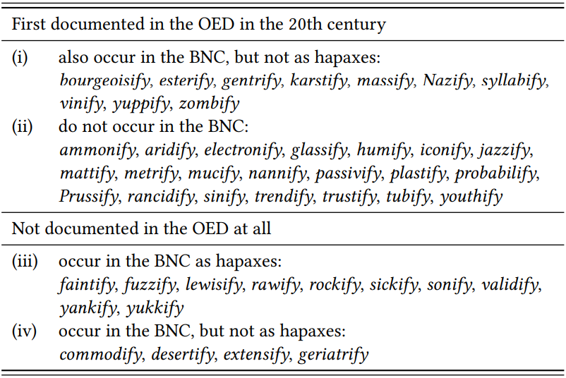
corpus data and dictionary data, we can increase coverage substantially even for moderately productive affixes.

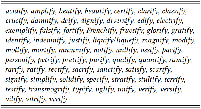
Let us now turn to the definition of \(\mathrm{established \space types}\). Given our definition of \(\mathrm{neologisms}\), established types would first have to be documented before the 20th century, so we could use the 420 types in the OED that meet this criterion (again, excluding prefixed forms). However, these 420 types contain many very rare or even obsolete forms, like duplify ‘to make double’, eaglify ‘to make into an eagle’ or naucify ‘to hold in low esteem’. Clearly, these are not “established” in any meaningful sense, so let us add the requirement that a type must occur in the BNC at least twice to count as established. Let us further limit the category to verbs first documented before the 19th century, in order to leave a clear diachronic gap between the established types and the productive types. This leaves the words in \(Table \text { } 9.9\).⁴

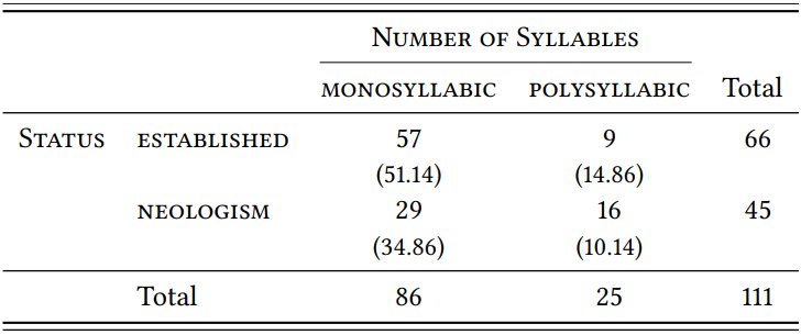
Let us now evaluate the hypotheses. \(Table \text { } 9.10\) shows the type frequencies for monosyllabic and polysyllabic stems in the two samples. In both cases, there is a preference for monosyllabic stems (as expected), but interestingly, this preference is less strong among the neologisms than among the established types and this difference is very significant (\(\chi^{2}\) = 7.37, df = 1, \(p\) < 0.01, \(\phi\) = 0.2577).

\(Table \text { } 9.9\): Control sample of established types with the suffix -ify.

\(Table \text { } 9.10\): Monosyllabic and bisyllabic stems with -ify

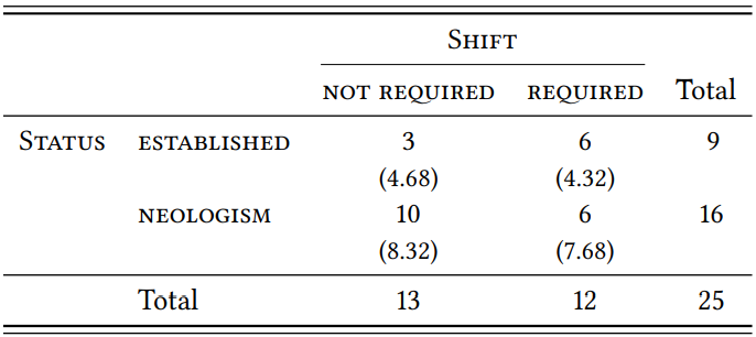
Given the fact that there is a significantly higher number of neologisms with polysyllabic stems than expected on the basis of established types, the second hypothesis becomes more interesting: does this higher number of polysyllabic stems correspond with a greater willingness to apply it to stems that then have to undergo stress shift (which would be contrary to our hypothesis, which assumes that there will be no difference between established types and neologisms)?

\(Table \text { } 9.11\) shows the relevant data: it seems that there might indeed be such a greater willingness, as the number of neologisms with polysyllabic stems requiring stress shift is higher than expected; however, the difference is not statistically significant ( \(\chi^{2}\) = 1.96, df = 1, \(p\) > 0.05, \(\phi\) = 0.28) (strictly speaking, we cannot use the \(\chi^{2}\) test here, since half of the expected frequencies are below 5, but Fisher’s exact test confirms that the difference is not significant).

\(Table \text { } 9.11\): Stress shift with polysyllabic stems with -ify

This case study demonstrates some of the problems and advantages of using corpora to identify neologisms in addition to existing dictionaries. It also constitutes an example of a purely type-based research design; note, again, that such a design is possible here because we are not interested in the type frequency of a particular affix under different conditions (in which case we would have to calculate a TTR to adjust for different sample sizes), but in the distribution of the variables \(\mathrm{Syllable \space Length}\) and \(\mathrm{Stress \space Shift}\) in two qualitatively different categories of types. Finally, note that the study comes to different conclusions than the impressionistic analysis in Plag (1999), so it demonstrates the advantages of strictly quantified designs.

9.2.1.2 Case study: Semantic differences between -ic and -ical

Affixes, like words, can be related to other affixes by lexical relations like synonymy, antonymy, etc. In the case of (roughly) synonymous affixes, an obvious research question is what determines the choice between them – for example, whether there are more fine-grained semantic differences that are not immediately apparent.

One way of approaching this question is to focus on stems that occur with both affixes (such as liqui(d) in liquidize and liquify/liquefy, scarce in scarceness and scarcity or electr- in electric and electrical) and to investigate the semantic contexts in which they occur – for example, by categorizing their collocates, analogous to the way Taylor (2003) categorizes collocates of high and tall (cf. Chapter 7, Section 7.2.2.1).

A good example of this approach is found in Kaunisto (1999), who investigates the pairs electric/electrical and classic/classical on the basis of the British Newspaper Daily Telegraph. Since his corpus is not accessible, let us use the LOB corpus instead to replicate his study for electric/electrical. It is a study with two nominal variables: \(\mathrm{Affix \space Variant}\) (with the values -ic and -ical), and \(\mathrm{Semantic \space Category}\) (with a set of values to be discussed presently). Note that this design can be based straightforwardly on token frequency, as we are not concerned with the relationship between the stem and the affix, but with the relationship between the stem-affix combination and the nouns modified by it. Put differently, we are not using the token frequency of a stem-affix combination, but of the collocates of words derived by a particular affix.

Kaunisto uses a mixture of dictionaries and existing literature to identify potentially interesting values for the variable \(\mathrm{Semantic \space Category}\); we will restrict ourselves to dictionaries here. Consider the definitions from six major dictionaries in (6) and (7):

6. electric
   1. connected with electricity; using, produced by or producing electricity (OALD)
   2. of or relating to electricity; operated by electricity (MW)
   3. working by electricity; used for carrying electricity; relating to electricity (MD)
   4. of, produced by, or worked by electricity (CALD)
   5. needing electricity to work, produced by electricity, or used for carrying electricity (LDCE)
   6. work[ing] by means of electricity; produced by electricity; designed to carry electricity; refer[ring] to the supply of electricity (Cobuild)
7. electrical
   1. connected with electricity; using or producing electricity (OALD)
   2. of or relating to electricity; operated by electricity (MW) [mentioned as a synonym under corresp. sense of electric]
   3. working by electricity; relating to electricity (MD)
   4. related to electricity (CALD, LDCE)
   5. work[ing] by means of electricity; supply[ing] or us[ing] electricity; energy ... in the form of electricity; involved in the production and supply of electricity or electrical goods (Cobuild)

MW treats the two words as largely synonymous and OALD distinguishes them only insofar as mentioning for electric, but not electrical, that it may refer to phenomena ‘produced by electricity’ (this is meant to cover cases like electric current/charge); however, since both words are also defined as referring to anything ‘connected with electricity’, this is not much of a differentiation (the entry for electrical also mentions electrical power/energy). Macmillan’s dictionary also treats them as largely synonymous, although it is pointed out specifically that electric refers to entities ‘carrying electricity’ (citing electric outlet/plug/cord). CALD and LDCE present electrical as a more general word for anything ‘related to electricity’, whereas they mention specifically that electric is used for things ‘worked by electricity’ (e.g. electric light/appliance) or ‘carrying electricity’ (presumably cords, outlets, etc.) and phenomena produced by electricity (presumably current, charge, etc.). Collins presents both words as referring to electric(al) appliances, with electric additionally referring to things ‘produced by electricity’, ‘designed to carry electricity’ or being related to the ‘supply of electricity’ and electrical additionally referring to ‘energy’ or entities ‘involved in the production and supply of electricity’ (presumably energy companies, engineers, etc.).

Summarizing, we can posit the following four broad values for our variable \(\mathrm{Semantic \space Category}\), with definitions that are hopefully specific enough to serve as an annotation scheme:

• \(\mathrm{devices}\) and appliances working by electricity (light, appliance, etc.)
• \(\mathrm{energy}\) in the form of electricity (power, current, charge, energy, etc.)
• the \(\mathrm{industry}\) researching, producing or supplying energy, i.e. companies and the people working there (company, engineer, etc.)
• \(\mathrm{circuits}\), broadly defined as entities producing or carrying electricity, including (cord, outlet, plug, but also power plant, etc.)

The definitions are too heterogeneous to base a specific hypothesis on them, but we might broadly expect electric to be more typical for the categories \(\mathrm{device}\) and \(\mathrm{circuit}\) and electrical for the category \(\mathrm{industry}\).

\(Table \text { } 9.12\) shows the token frequency with which nouns from these categories are referred to as electric or electrical in the LOB corpus; in order to understand how these nouns were categorized, it also lists all types found for each category (one example was discarded because it was metaphorical).

The difference between electric and electrical is significant overall (\(\chi^{2}\) = 12.68, df = 3, \(p\) < 0.01, \(\phi\) = 0.2869), suggesting that the two words somehow differ with

\(Table \text { } 9.12\): Entities described as electric or electrical in the LOB corpus

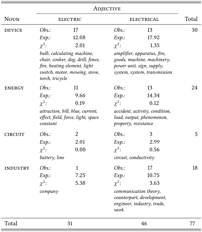
respect to their preferences for these categories. Since we are interested in the nature of this difference, it is much more insightful to look at the \(\chi^{2}\) components individually. This gives us a better idea where the overall significant difference comes from. In this case, it comes almost exclusively from the fact that electrical is indeed associated with the research and supply of electricity (\(\mathrm{industry}\)), although there is a slight preference for electric with nouns referring to devices. Generally, the two words seem to be relatively synonymous, at least in 1960s British English.

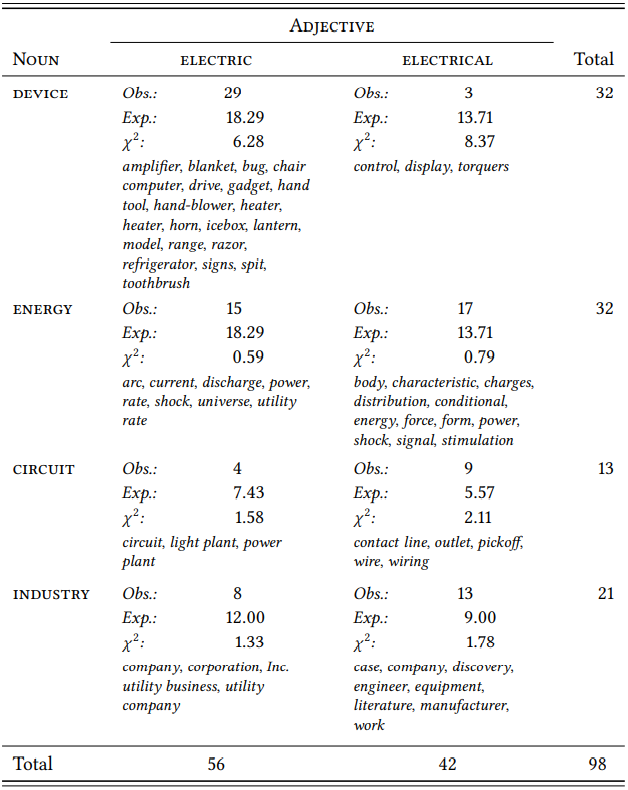
Let us repeat the study with the BROWN corpus. \(Table \text { } 9.13\) lists the token frequencies for the individual categories and, again, all types found for each category.

Again, the overall difference between the two words is significant and the effect is slightly stronger than in the LOB corpus (\(\chi^{2}\) = 22.83, df = 3, \(p\) < 0.001, \(\phi\) = 0.3413), suggesting a stronger differentiation between them. Again, the most interesting question is where the effect comes from. In this case, devices are much more frequently referred to as electric and less frequently as electrical than expected, and, as in the LOB corpus, the nouns in the category industry are more frequently referred to as electrical and less frequently as electric than expected (although not significantly so). Again, there is no clear difference with respect to the remaining two categories.

Broadly speaking, then, one of our expectations is borne out by the British English data and one by the American English data. We would now have to look at larger corpora to see whether this is an actual difference between the two varieties or whether it is an accidental feature of the corpora used here. We might also want to look at more modern corpora – the importance of electricity in our daily lives has changed quite drastically even since the 1960s, so the words may have specialized semantically more clearly in the meantime. Finally, we would look more closely at the categories we have used, to see whether a different or a more fine-grained categorization might reveal additional insights (Kaunisto (1999) goes on to look at his categories in more detail, revealing more fine-grained differences between the words).

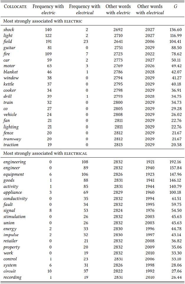
Of course, this kind of investigation can also be designed as an inductive study of differential collocates (again, like the study of synonyms such as high and tall). Let us look at the nominal collocates of electric and electrical in the BNC. \(Table \text { } 9.14\) shows the results of a differential-collocate analysis, calculated on the basis of all occurrences of electric/al in the BNC that are directly followed by a noun.

\(Table \text { } 9.13\): Entities described as electric or electrical in the BROWN corpus

The results largely agree with the preferences also uncovered by the more careful (and more time-consuming) categorization of a complete data set, with one crucial difference: there are members of the category \(\mathrm{device}\) among the significant differential collocates of both variants. A closer look reveals a systematic difference within this category: the \(\mathrm{device}\) collocates of electric refer to specific devices (such as light, guitar, light, kettle, etc.); in contrast, the \(\mathrm{device}\) collocates of electrical refer to general classes of devices (equipment, appliance, system). This difference was not discernible in the LOB and BROWN datasets (presumably because they were too small), but it is discernible in the data set used by Kaunisto (1999), who posits corresponding subcategories. Of course, the BNC is a much more recent corpus than LOB and BROWN, so, again, a diachronic comparison would be interesting.

There is an additional pattern that would warrant further investigation: there are collocates for both variants that correspond to what some of the dictionaries we consulted refer to as ‘produced by energy’: shock, field and fire for electric and signal, energy, impulse for electrical. It is possible that electric more specifically characterizes phenomena that are caused by electricity, while electrical characterizes phenomena that manifest electricity.

The case study demonstrates, then, that a differential-collocate analysis is a good alternative to the manual categorization and category-wise comparison of all collocates: it allows us to process very large data sets very quickly and then focus on the semantic properties of those collocates that are shown by the statistical analysis to differentiate between the variants.

We must keep in mind, however, that this kind of study does not primarily uncover differences between affixes, but differences between specific word pairs containing these affixes. They are, as pointed out above, essentially lexical studies of near-synonymy. Of course, it is possible that by performing such analyses for a large number of word pairs containing a particular affix pair, general semantic differences may emerge, but since we are frequently dealing with highly lexicalized forms, there is no guarantee for this. Gries (2001; 2003b) has shown that -ic/-ical pairs differ substantially in the extent to which they are synonymous; for example, he finds substantial difference in meaning for politic/political or poetic/poetical, but much smaller differences, for example, for bibliographic/ bibliographical, with electric/electrical somewhere in the middle. Obviously, the two variants have lexicalized independently in many cases, and the specific differences in meaning resulting from this lexicalization process are unlikely to fall into clear general categories.

\(Table \text { } 9.14\): Differential nominal collocates of electric and electrical in the BNC

9.2.1.3 Case study: Phonological differences between -ic and -ical

In an interesting but rarely-cited paper, Or (1994) collects a number of hypotheses about semantic and, in particular, phonological factors influencing the distribution of -ic and -ical that she provides impressionistic corpus evidence for but does not investigate systematically. A simple example is the factor \(\mathrm{Length}\): Or hypothesizes that speakers will tend to avoid long words and choose the shorter variant -ic for long stems (in terms of number of syllables). She reports that “a survey of a general vocabulary list” corroborates this hypothesis but does not present any systematic data.

Let us test this hypothesis using the LOB corpus. Since this is a written corpus, let us define \(\mathrm{Length}\) in terms of letters and assume that this is a sufficiently close approximation to phonological length. \(Tables \text { } 9.15\) and \(9.16\) lists all types with the two suffixes from LOB in decreasing order of length; note that since the point here is to show the influence of length on suffix choice, prefixed stems, compound stems, etc. are included in their full form (the lists are included in a more readable format in the Supplementary Online Materials, file U7BR).

We can test the hypothesis based on the mean length of the two samples using a \(t\)-test, or by ranking them by length using the \(U\) test. As mentioned in Chapter 6, word length (however we measure it) rarely follows a normal distribution, so the \(U\) test would probably be the better choice in this case, but let us use the \(t\)-test for the sake of practice (the data are there in full, if you want to calculate a \(U\) test).

There are 373 stem types occurring with -ic in the LOB corpus, with a mean length of 7.32 and a sample variance of 5.72; there are 153 stem types occurring with -ical, with a mean length of 6.60 and a sample variance of 4.57. Applying the formula in (15) from Chapter 6, we get a \(t\)-value of 2.97. There are 314.31 degrees of freedom in our sample (as calculated using the formula in 16), which means that \(p\) < 0.001. In other words, length (as measured in letters) seems to have an influence on the choice between the two affixes, with longer stems favoring -ic.

This case study has demonstrated the use of a relatively simple operationalization to test a hypothesis about phonological length. We have used samples of types rather than samples of tokens, as we wanted to determine the influence of stem length on affix choice – in this context, the crucial question is how many stems of a given length occur with a particular affix variant, but it does not matter how often a particular stem does so. However, if there was more variation between the two suffixes, the frequency with which a particular stem is used with a particular affix might be interesting, as it would allow us to approach the question by ranking stems in terms of their preference and then correlating this ranking with their length.

\(Table \text { } 9.15\): Adjectives with -ic by length (LOB)

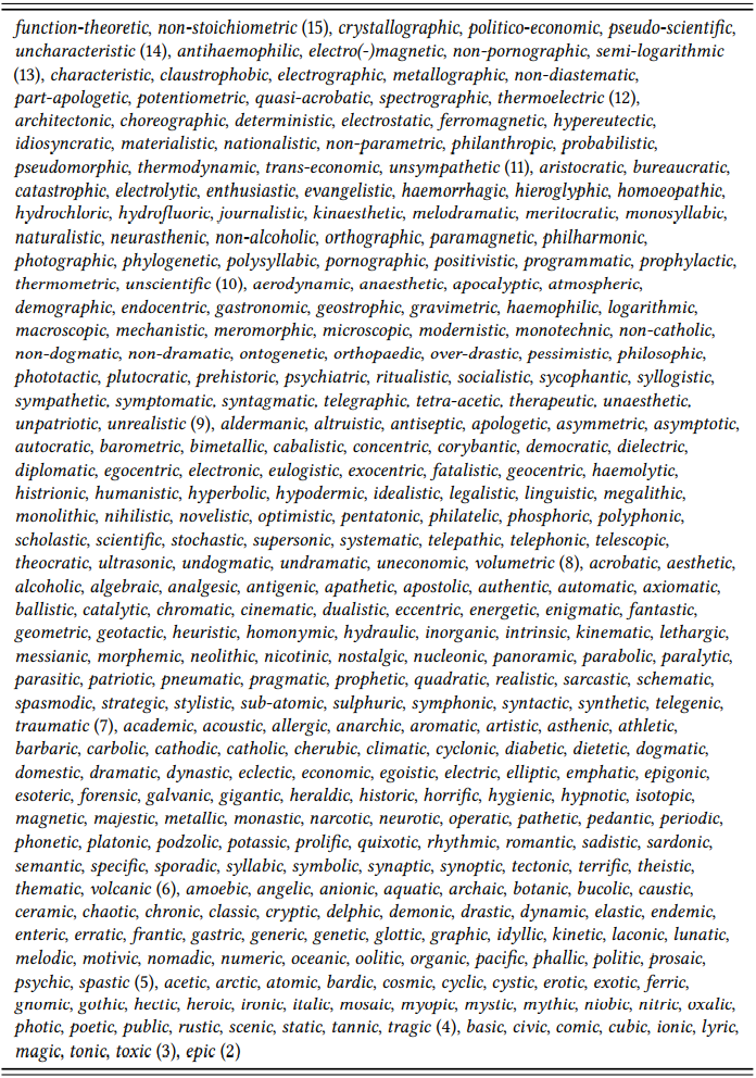
\(Table \text { } 9.16\): Adjectives with -ical by length (LOB)

9.2.1.4 Case study: Affix combinations

It has sometimes been observed that certain derivational affixes show a preference for stems that are already derived by a particular affix. For example, Lindsay (2011) and Lindsay & Aronoff (2013)show that while -ic is more productive in general than -ical, -ical is more productive with stems that contain the affix -olog- (for example, morphological or methodological). Such observations are interesting from a descriptive viewpoint, as such preferences need to be taken into account, for example, in dictionaries, in teaching word-formation to non-native speakers or when making or assessing stylistic choices. They are also interesting from a theoretical perspective, first, because they need to be modeled and explained within any morphological theory, and second, because they may interact with other factors in a number of different ways.

For example, Case Study 9.2.1.3 demonstrates that longer stems generally seem to prefer the variant -ic; however, the mean length of derived stems is necessarily longer than that of non-derived stems, so it is puzzling, at first glance, that stems with the affix -olog- should prefer -ical. Of course, -olog- may be an exception, with derived stems in general preferring the shorter -ic; however, we would still need to account for this exceptional behavior.

But let us start more humbly by laying the empirical foundations for such discussions and test the observation by Lindsay (2011) and Lindsay & Aronoff (2013). The authors themselves do so by comparing the ratio of the two suffixes for stems that occur with both suffixes. Let us return to their approach later, and start by looking at the overall distribution of stems with -ic and -ical.

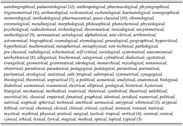
First, though, let us see what we can find out by looking at the overall distribution of types, using the four-million-word BNC Baby. Once we remove all prefixes and standardize the spelling, there are 846 types for the two suffixes. There is a clear overall preference for -ic (659 types) over -ical (187 types) (incidentally, there are only 54 stems that occur with both suffixes). For stems with -(o)log-, the picture is drastically different: there is an overwhelming preference for -ical (55 types) over -ic (3 types). We can evaluate this difference statistically, as shown in \(Table \text { } 9.17\).

\(Table \text { } 9.17\): Preference of stems with -olog- for -ic and -ical

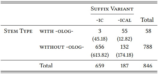
Unsurprisingly, the difference between stems with and without the affix -olog- is highly significant (\(\chi^{2}\) = 191.27, df = 1, \(p\) < 0.001) – stems with -olog- clearly favor the variant -ical against the general trend.

As mentioned above, this could be due specifically to the affix -olog-, but it could also be a general preference of derived stems for -ical. In order to determine this, we have to look at derived stems with other affixes. There are a number of other affixes that occur frequently enough to make them potentially interesting, such as -ist-, as in statistic(al) (-ic vs. -ical: \(\frac{74}{2}\)), -graph-, as in geographic(al) (\(\frac{19}{8}\)), or -et-, as in arithmetic(al) (\(\frac{32}{9}\)). Note that all of them have more types with -ic, which suggests that derived stems in general, possibly due to their length, prefer -ic and that -olog- really is an exception.

But there is a methodological issue that we have to address before we can really conclude this. Note that we have been talking of a “preference” of particular stems for one or the other suffix, but this is somewhat imprecise: we looked at the total number of stem types with -ic and -ical with and without additional suffixes. While differences in number are plausibly attributed to preferences, they may also be purely historical leftovers due to the specific history of the two suffixes (which is rather complex, involving borrowing from Latin, Greek and, in the case of -ical, French). More convincing evidence for a productive difference in preferences would come from stems that take both -ic and -ical (such as electric/al, symmetric/al or numeric/al, to take three examples that display a relatively even distribution between the two): for these stems, there is obviously a choice, and we can investigate the influence of additional affixes on that choice.

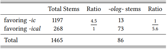
Lindsay (2011) and Lindsay & Aronoff (2013) focus on precisely these stems, checking for each one whether it occurs more frequently with -ic or with -ical and calculating the preference ratio mentioned above. They then compare the ratio of all stems to that of stems with -olog- (see \(Table \text { } 9.18\)).

\(Table \text { } 9.18\): Stems favoring -ic or -ical in the COCA (Lindsay 2011: 194)

The ratios themselves are difficult to compare statistically, but they are clearly the right way of measuring the preference of stems for a particular suffix. So let us take Lindsay and Aronoff’s approach one step further: Instead of calculating the overall preference of a particular type of stem and comparing it to the overall preference of all stems, let us calculate the preference for each stem individually. This will give us a preference measure for each stem that is, at the very least, ordinal.⁵ We can then rank stems containing a particular affix and stems not containing that affix (or containing a specific different affix) by their preference for one or the other of the suffix variants and use the Mann-Whitney U-test to determine whether the stems with -olog- tend to occur towards the -ical end of the ranking. That way we can treat preference as the matter of degree that it actually is, rather than as an absolute property of stems.

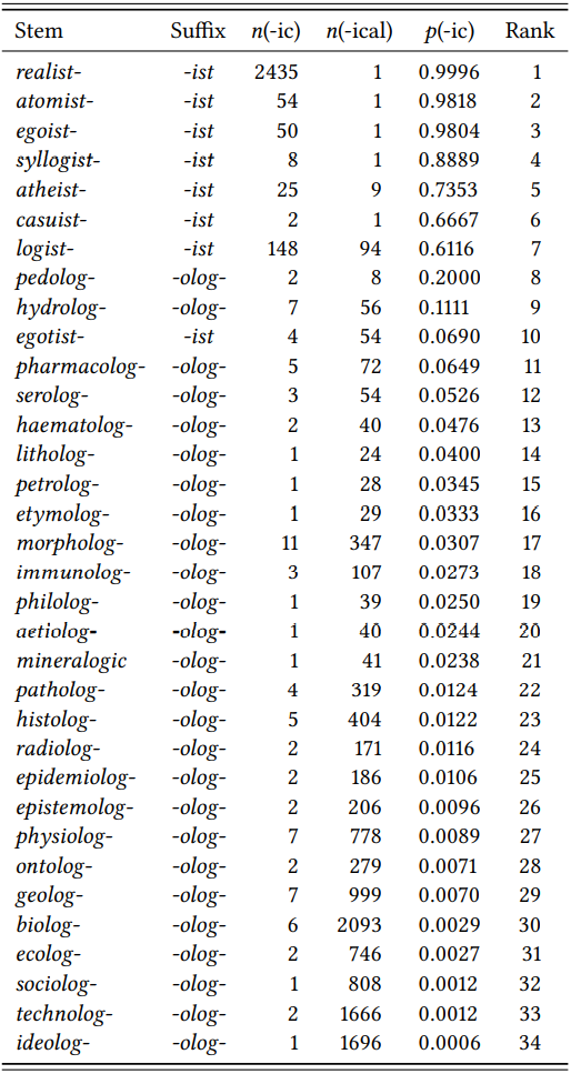
The BNC Baby does not contain enough derived stems that occur with both suffix variants, so let us focus on two specific suffixes and extract the relevant data from the full BNC. Since -ist is roughly equal to -olog- in terms of type frequency, let us choose this suffix for comparison. \(Table \text { } 9.19\) shows the 34 stems containing either of these suffixes, their frequency of occurrence with the variants -ic and -ical, the preference ratio for -ic, and the rank.

The different preferences of stems with -ist and -olog- are very obvious even from a purely visual inspection of the table: stems with the former occur at the top of the ranking, stems with the latter occur at the bottom and there is almost no overlap. This is reflected clearly in the median ranks of the two stem types: the median for -ist is 4.5 (\(N\) = 8,rank sum = 38), the median for -olog- is 21.5 (\(N\) = 26,rank sum = 557). A Mann-Whitney U test shows that this difference is highly significant (\(U\) = 2, \(N_{1}\) = 8, \(N_{2}\) = 26, \(p\) < 0.001).

Now that we have established that different suffixes may, indeed, display different preferences for other suffixes (or suffix variants), we could begin to answer the question why this might be the case. In this instance, the explanation is likely found in the complicated history of borrowings containing the suffixes in question. The point of this case study was not to provide such an explanation but to show how an empirical basis can be provided using token frequencies derived from linguistic corpora.

9.2.2 Morphemes and demographic variables

There are a few studies investigating the productivity of derivational morphemes across language varieties (e.g., medium or genre), across groups defined by sex, education and/or class, or across varieties. This is an extremely interesting area of research that may offer valuable insights into the very nature of morphological richness and productivity, allowing us, for example, to study potential differences between regular, presumably subconscious applications of derivational rules and the deliberate coining of words. Despite this, it is an area that has not been studied too intensively, so there is much that remains to be discovered.

9.2.2.1 Case study: Productivity and genre

Guz (2009) studies the prevalence of different kinds of nominalization across genres. The question whether the productivity of derivational morphemes differs across genres is a very interesting one, and Guz presents a potentially more

\(Table \text { } 9.19\): Preferences of stems containing -ist and -olog- for the suffix variants -ic and -ical (BNC)

detailed analysis than previous studies in that he looks at the prevalence of different stem types for each affix, so that qualitative as well as quantitative differences in productivity could, in theory, be studied. In practice, unfortunately, the study offers preliminary insights at best, as it is based entirely on token frequencies, which, as discussed in Section 9.1 above, do not tell us anything at all about productivity.

We will therefore look at a question inspired by Guz’s study, and use the TTR and the HTR to study the relative importance and productivity of the nominalizing suffix -ship (as in friendship, lordship, etc.) in newspaper language and in prose fiction. The suffix -ship is known to have a very limited productivity, and our hypothesis (for the sake of the argument) will be that it is more productive in prose fiction, since authors of fiction are under pressure to use language creatively (this is not Guz’s hypothesis; his study is entirely explorative).

The suffix has a relatively high token frequency: there are 2862 tokens in the fiction section of the BNC, and 7189 tokens in the newspaper section (including all sub-genres of newspaper language, such as reportage, editorial, etc.) (the data are provided in the Supplementary Online Material, file LAF3). This difference is not due to the respective sample sizes: the fiction section in the BNC is much larger than the newspaper section; thus, the difference token frequency would suggest that the suffix is more important in newspaper language than in fiction. However, as extensively discussed in Section 9.1.1, token frequency cannot be used to base such statements on. Instead, we need to look at the type-token ratio and the hapax-token ratio.

To get a first impression, consider \(Figure \text { } 9.4\), which shows the growth of the TTR (left) and HTR (right) in the full \(\mathrm{fiction}\) and \(\mathrm{newspaper}\) sections of the BNC.

Both the TTR and the HTR suggest that the suffix is more productive in fiction: the ratios rise faster in \(\mathrm{fiction}\) than in \(\mathrm{newspapers}\) and remain consistently higher as we go through the two sub-corpora. It is only when the tokens have been exhausted in the fiction subcorpus but not in the newspaper subcorpus, that the ratios in the latter slowly catch up. This broadly supports our hypothesis, but let us look at the genre differences more closely both qualitatively and quantitatively.

In order to compare the two genres in terms of the type-token and hapaxtoken ratios, they need to have the same size. The following discussion is based on the full data from the fiction subcorpus and a subsample of the newspaper corpus that was arrived at by deleting every second, then every third and finally every 192nd example, ensuring that the hits in the sample are spread through the entire newspaper subcorpus.

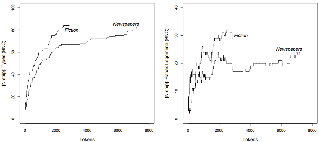
\(Figure \text { } 9.4\): Nouns with the suffix -ship in the Genre categories fiction and newspapers (BNC)

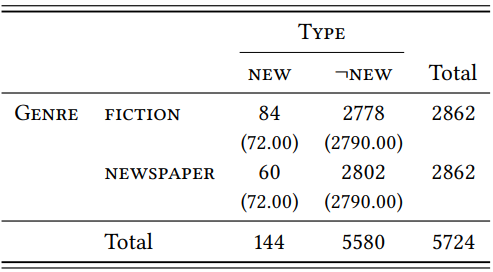
Let us begin by looking at the types. Overall, there are 96 different types, 48 of which occur in both samples (some examples of types that frequent in both samples are relationship (the most frequent word in the fiction sample), championship (the most frequent word in the news sample), friendship, partnership, lordship, ownership and membership. In addition, there are 36 types that occur only in the prose sample (for example, churchmanship, dreamership, librarianship and swordsmanship) and 12 that occur only in the newspaper sample (for example, associateship, draughtsmanship, trusteeship and sportsmanship). The number of types exclusive to each genre suggests that the suffix is more important in \(\mathrm{fiction}\) than in \(\mathrm{newspapers}\).

The TTR of the suffix in newspaper language is \(\frac{60}{2862}\) = 0.021, and the HTR is \(\frac{20}{2862}\) = 0.007. In contrast, the TTR in fiction is \(\frac{84}{2862}\) = 0.0294, and the HTR is \(\frac{29}{2862}\) = 0.0101. Although the suffix, as expected, is generally not very productive, it is more productive in fiction than in newspapers. As \(Table \text { } 9.20\) shows, this difference is statistically significant in the sample (\(\chi^{2}\) = 4.1, df = 1, \(p\) < 0.005). This corroborates our hypothesis, but note that it does not tell us whether the higher productivity of -ship is something unique about this particular morpheme, or whether fiction generally has more derived words due to a higher overall lexical richness. To determine this, we would have to look at more than one affix.

Let us now turn to the hapax legomena. These are so rare in both genres that the difference in TTR is not statistically significant, as \(Table \text { } 9.21\) shows (\(\chi^{2}\) = 1.67, df = 1, \(p\) = 0.1966). We would need a larger corpus to see whether the difference would at some point become significant.

\(Table \text { } 9.20\): Types with -ship in prose fiction and newspapers

\(Table \text { } 9.21\): Hapaxes with -ship in prose fiction and newspapers

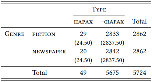
To conclude this case study, let us look at a particular problem posed by the comparison of the same suffix in two genres with respect to the HTR. At first glance – and this is what is shown in \(Table \text { } 9.21\) – there seem to be 29 hapaxes in fiction and 20 in prose. However, there is some overlap: the words generalship, headship, managership, ministership and professorship occur as hapax legomena in both samples; other words that are hapaxes in one subsample occur several times in the other, such as brinkmanship, which is a hapax in fiction but occurs twice in the newspaper sample, or acquaintanceship, which is a hapax in the newspaper sample but occurs 15 times in fiction.

It is not straightforwardly clear whether such cases should be treated as hapaxes. If we think of the two samples as subsamples of the same corpus, it is very counterintuitive to do so. It might be more reasonable to count only those words as hapaxes whose frequency in the combined subsamples is still one. However, the notion “hapax” is only an operational definition for neologisms, based on the hope that the number of hapaxes in a corpus (or sub-corpus) is somehow indicative of the number of productive coinages. We saw in Case Study 9.2.1.1 that this is a somewhat vain hope, as the correlation between neologisms and hapaxes is not very impressive.

Still, if we want to use this operational definition, we have to stick with it and define hapaxes strictly relative to whatever (sub-)corpus we are dealing with. If we extend the criterion for hapax-ship beyond one subsample to the other, why stop there? We might be even stricter and count only those words as hapaxes that are still hapaxes when we take the entire BNC into account. And if we take the entire BNC into account, we might as well count as hapaxes only those words that occur only once in all accessible archives of the language under investigation. This would mean that the hapaxes in any sample would overwhelmingly cease to be hapaxes – the larger our corpus, the fewer hapaxes there will be. To illustrate this: just two words from the fiction sample retain their status as hapax legomena if we search the Google Books collection: impress-ship, which does not occur at all (if we discount linguistic accounts which mention it, such as Trips (2009), or this book, once it becomes part of the Google Books archive), and cloudship, which does occur, but only referring to water- or airborne vehicles. At the same time, the Google Books archive contains hundreds (if not thousands) of hapax legomena that we never even notice (such as Johnship ‘the state of being the individual referred to as John’). The idea of using hapax legomena is, essentially, that a word like mageship, which is a hapax in the fiction sample, but not in the Google Books archive, somehow stands for a word like Johnship, which is a true hapax in the English language.

This case study has demonstrated the potential of using the TTR and the HTR not as a means of assessing morphological richness and productivity as such, but as a means of assessing genres with respect to their richness and productivity. It has also demonstrated some of the problems of identifying hapax legomena in the context of such cross-variety comparisons. As mentioned initially, there are not too many studies of this kind, but Plag (1999) presents a study of productivity across written and spoken language that is a good starting point for anyone wanting to fill this gap

9.2.2.2 Case study: Productivity and speaker sexds

Morphological productivity has not traditionally been investigated from a sociolinguistic perspective, but a study by Säily (2011) suggests that this may be a promising field of research. Säily investigates differences in the productivity of the suffixes -ness and -ity in the language produced by men and women in the BNC. She finds no difference in productivity for -ness, but a higher productivity of -ity in the language produced by men (cf. also Säily & Suomela 2009 for a diachronic study with very similar results). She uses a sophisticated method involving the comparison of the suffixes’ type and hapax growth rates, but let us replicate her study using the simple method used in the preceding case study, beginning with a comparison of type-token ratios.

The BNC contains substantially more speech and writing by male speakers than by female speakers, which is reflected in differences in the number of affix tokens produced by men and women: for -ity, there are 2562 tokens produced by women and 8916 tokens produced by men; for -ness, there are 616 tokens produced by women and 1154 tokens produced by men (note that unlike Säily, I excluded the words business and witness, since they did not seem to me to be synchronically transparent instances of the affix). To get samples of equal size for each affix, random subsamples were drawn from the tokens produced by men.

Based on these subsamples, the type-token ratios for -ity are 0.0652 for men and 0.0777 for women; as \(Table \text { } 9.22\) shows, this difference is not statistically significant (\(\chi^{2}\) = 3.01, df = 1, \(p\) < 0.05, \(\phi\) = 0.0242).

\(Table \text { } 9.22\): Types with -ity in male and female speech (BNC)

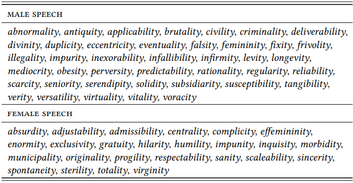
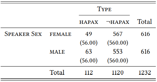
The type-token ratios for -ness are much higher, namely 0.1981 for women and 0.2597 for men. As \(Table \text { } 9.23\) shows, the difference is statistically significant, although the effect size is weak (\(\chi^{2}\) = 5.37, df = 1, \(p\) < 0.05, \(\phi\) = 0.066).

Note that Säily investigates spoken and written language separately and she also includes social class in her analysis, so her results differ from the ones presented here; she finds a significantly lower HTR for -ness in lower-class women’s speech in the spoken subcorpus, but not in the written one, and a significantly lower HTR for -ity in both subcorpora. This might be due to the different methods used, or to the fact that I excluded business, which is disproportionally frequent

\(Table \text { } 9.23\): Types with -ness in male and female speech (BNC)

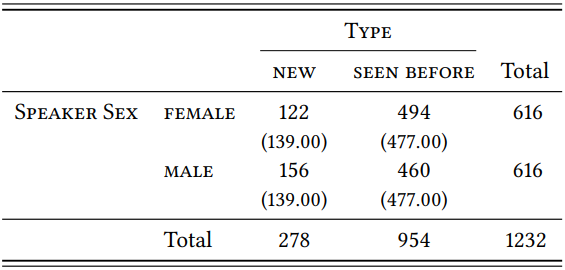
in male speech and writing in the BNC and would thus reduce the diversity in the male sample substantially. However, the type-based differences do not have a very impressive effect size in our design and they are unstable across conditions in Säily’s, so perhaps they are simply not very substantial.

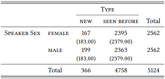
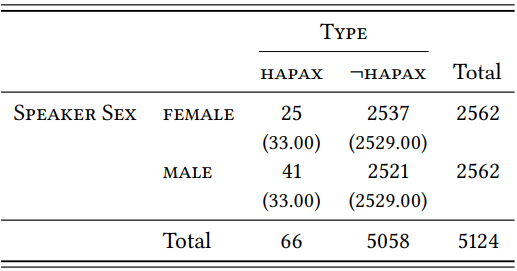
Let us turn to the HTR next. As before, we are defining what counts as a hapax legomenon not with reference to the individual subsamples of male and female speech, but with respect to the combined sample. \(Table \text { } 9.24\) shows the hapaxes for -ity in the male and female samples. The HTRs are very low, suggesting that -ity is not a very productive suffix: 0.0099 in female speech and 0.016 in male speech.

\(Table \text { } 9.24\): Hapaxes with -ity in sampes of male and female speech (BNC)

Although the difference in HTR is relatively small, \(Table \text { } 9.25\) shows that it is statistically significant, albeit again with a very weak effect size (\(\chi^{2}\) = 3.93, df = 1, \(p\) < 0.05, \(\phi\) = 0.0277).

\(Table \text { } 9.25\): Hapax legomena with -ity in male and female speech (BNC)

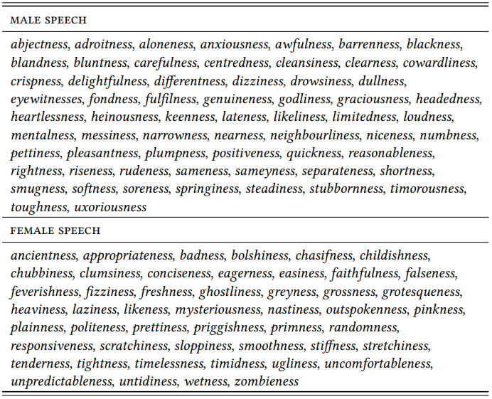
\(Table \text { } 9.26\) shows the hapaxes for -ness in the male and female samples. The HTRs are low, but much higher than for -ity, 0.0795 for women and 0.1023 for men.

As \(Table \text { } 9.27\) shows, the difference in HTRs is not statistically significant, and the effect size would be very weak anyway (\(\chi^{2}\) = 1.93, df = 1, \(p\) > 0.05, \(\phi\) = 0.0395).

In this case, the results correspond to Säily’s, who also finds a significant difference in productivity for -ity, but not for -ness.

This case study was meant to demonstrate, once again, the method of comparing TTRs and HTRs based on samples of equal size. It was also meant to draw attention to the fact that morphological productivity may be an interesting area of research for variationist sociolinguistics; however, it must be pointed out that it would be premature to conclude that men and women differ in their productive use of particular affixes; as Säily herself points out, men and women are not only represented unevenly in quantitative terms (with a much larger proportion of male language included in the BNC), but also in qualitative terms (the language varieties with which they are represented differ quite strikingly). Thus, this may actually be another case of different degrees of productivity in different language varieties (which we investigated in the preceding case study).

\(Table \text { } 9.26\): Hapaxes with -ness in samples of male and female speech (BNC)

\(Table \text { } 9.27\): Hapax legomena with -ness in male and female speech (BNC)

__________________________

³This is a simplification: stress-shift only occurs with unstressed closed syllables or sequence of two unstressed syllables (SYLlable – sylLAbify). Occasionally, stem-final consonants are deleted (as in liquid – liquify); cf. Plag (1999) for a more detailed discussion.
⁴Interestingly, leaving out words coined in the 19th century does not make much of a difference: although the 19th century saw a large number of coinages (with 138 new types it was the most productive century in the history of the suffix), few of these are frequent enough today to occur in the BNC; if anything, we should actually extend our definition of neologisms to include the 19th century.
⁵In fact, measures derived in this way are cardinal data, as the value can range from 0 to 1 with every possible value in between; it is safer to treat them as ordinal data, however, because we don’t know whether such preference values are normally distributed. In fact, since they are based on word frequency data, which we know not to be normally distributed, it is a fair guess that the preference data are not normally distributed.