The basic idea of the Theory of Consumer Behavior is simple: Given a budget constraint, the consumer buys a combination of goods and services that maximizes satisfaction, which is captured by a utility function. By changing the price of a particular item, ceteris paribus (everything else held constant), we derive a demand curve for that item.
Setting up and solving the consumer’s utility maximization problem takes some time. We will proceed slowly and carefully. This chapter focuses on the budget constraint and how it changes when prices or income change.
What can be afforded is obviously a key factor in predicting buying behavior, but it is only part of the story. With the budget constraint alone, we cannot answer the question of how much the consumer wants to buy of each product because we are not incorporating any information about the utility gained by consumption. After we understand the budget constraint, we will model the consumer’s likes and dislikes. We can then put the constraint and utility components together and solve the model.
The Budget Constraint in Equation Form
The budget constraint can be expressed mathematically like this:
\(p_{1}x_{1} + p_{2}x_{2} \le m\)
This equation says that the sum of the amount of money spent on good \(x_{1}\), which is the price of \(x_{1}\) times the number of units purchased, or \(p_{1}x_{1}\), and the amount spent on good \(x_{2}\), which is \(p_{2}x_{2}\), must be less than or equal to the amount of income, m (for money), the consumer has available.
Obviously, the model would be more realistic if we had many products that the consumer could buy, but the gain in realism is not worth the additional cost in computational complexity. We can easily let \(x_{2}\) stand for “all other goods.”
Another simplification allows us to transform the inequality in the equation to a strict equality. We will assume that no time elapses so there is no saving (not spending all of the income available) or borrowing. In other words, the consumer lives for a nanosecond – buying, consuming, and dying the same instant. Once again, this assumption is not as severe as it first looks. We can incorporate saving and borrowing in this model by defining one good as present consumption and the other as future consumption. We will use this modeling technique in a future application.
Since we know we will always spend all of our income, the budget constraint equation can be written with an equal sign, like this
\(p_{1}x_{1} + p_{2}x_{2} = m\)
Since we will want to draw a graph, we can write in the form of the equation of a line (\(y = mx + b\)) via a little algebraic manipulation:
The intercept, \(m/p_{2}\), is interpreted as the maximum amount of \(p_{2}\) that the consumer can afford. By buying no \(x_{1}\) and spending all income on \(x_{2}\), the most the consumer can buy is \(m/p_{2}\) units of good 2.
The slope, \(-p_{1}/p_{2}\), also has a convenient interpretation: It states the rate at which the market requires the consumer to give up \(x_{2}\) in order to acquire \(x_{1}\). This is easy to see if you remember that the slope of a line is simply the rise (\(\Delta x_{2}\)) over the run (\(\Delta x_{1}\)). Then,
STEP Open the Excel workbook BudgetConstraint.xls, read the Intro sheet, and then go to the Properties sheet to see the budget constraint.
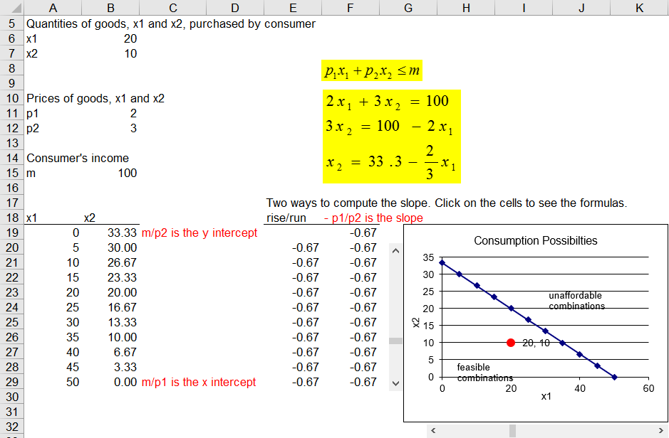
Figure 1.1 shows the organization of the sheet. As you can see, the consumer chooses the amounts of goods 1 and 2 to purchase, given prices and income.
Figure 1.1: The budget line.
Source: BudgetConstraint.xls!Properties
With \(p_{1}\) = $2/unit, \(p_{2}\) = $3/unit and \(m\) = $100, the equation of the budget line can be computed.
STEP Click on the scroll bars to see the red dot (which represents the consumption bundle), move around in the chart.
By rewriting the budget constraint equation as a line and then graphing it, we have a geometric representation of the consumer’s consumption possibilities. All points inside or on the budget line are feasible. Points northeast of the budget line are unaffordable.
By clicking the scroll bars you can easily see that the consumer has many feasible points. The big question is, Which one of these many affordable combinations will be chosen? We cannot answer that question with the budget constraint alone. We need to know how much the consumer likes the two goods. The constraint is simply about feasible options.
Changes in the Budget Line – Pivots and Shifts
STEP Proceed to the Changes sheet.
The idea here is that changes in prices cause the budget line to pivot or rotate, altering the slope, but keeping one of the intercepts the same. Note that changes in income produce a different result, shifting the budget line in or out, leaving the slope unchanged.
STEP To see how the budget line pivots, experiment with cell K9 (the price of good 1). Change it from 2 to 5.
The chart changes to reveal a new budget line. The budget line has rotated around the y intercept because if the consumer decided to spend all income on \(x_{2}\), the amount that could be purchased would remain the same.
If you lower the price of good 1, the budget line swings out. Confirm that this is true.
STEP Changing cell K10 alters the budget line by changing the price of good 2. Once again, change values in the cell to see the effect on the budget line.
STEP Next, click the button to return the sheet to its initial values and work with cell K13. Cut income in half. The effect is dramatically different. Instead of rotating, the budget line has shifted in. The slope remains the same because prices have not changed. Increasing income shifts the budget line out.
This concludes the basics of budget lines. It is worth spending a little time playing with cells K9, K10, and K13 to reinforce understanding of the way budget lines move when there is a change in a price or income. These shocks will be used again when we examine how a consumer’s optimal decision changes when prices or income change.
Remember the key lesson: Change in price rotates the budget line, but change in income shifts it.
Funky Budget Lines
In addition to the standard, linear budget constraint, there are many more complicated scenarios facing consumers. To give you a taste of the possibilities, let us review two examples.
STEP Proceed to the Rationing sheet.
In this example, in addition to the usual income constraint, the consumer is allowed a maximum amount of one of the goods. Thus, a second constraint (a vertical line) has been added. When the maximum is above the \(x_{1}\) intercept (50 units), this second constraint is said to be nonbinding. As you can see from the sheet, when the maximum amount constraint is binding, it lops off a portion of the budget line.
STEP Change cell E13 to see how changing the rationed amount affects the budget constraint.
As we increase the amount of the subsidy, the horizontal line is extended. The downward sloping part has the same slope, but it is pushed outwards,
STEP Proceed to the Subsidy sheet.
In this example, in addition to the usual income constraint, the consumer is given a subsidy in the form of a fixed amount of the good.
Food stamps are classic example of subsidies. Suppose the consumer has $100 of income, but is given $20 in food stamps (which can only be spent on food), and food (\(x_{1}\)) is priced at $2/unit. Then the budget constraint has a horizontal segment from 0 to 10 units of food because the most \(x_{2}\) (other goods) that can be purchased remains at \(m\)/\(p_{2}\) from 0 to 10 units of food (since food stamps cannot be used to buy other goods).
STEP Change cell E13 to see how changing the given amount of food (which is the dollar amount of food stamps divided by the price of food) affects the budget constraint.
Summary: Consumption Possibilities
The budget constraint is a key component of the optimization problem facing the consumer. Graphing the constraint lets us see the consumer’s options. Just like a production possibilities frontier tells us what an economy can produce, the budget constraint shows what a consumer can buy. Any combination on or under the constraint is a feasible option. Points beyond the constraint are unattainable.
Changing prices has a different effect on the constraint than changing income. If prices change, the budget line pivots, swings, and rotates (pick your favorite word and remember it) around the intercept. A change in income, however, shifts the line (out or in) and leaves the slope unaffected.
The basic budget constraint is a line, but there are many other scenarios faced by consumers in which the constraint can be kinked or nonlinear. Subsidies (like food stamps) can be incorporated into the basic model. This flexibility is one of the powerful features of the Theory of Consumer Behavior.
The constraint is just one part of the consumer’s optimization problem. The desirability of goods and services, also known as tastes and preferences, is another important part. The next chapter explains how we model satisfaction from consuming goods and services.
Exercises
Use Excel to create a chart of a budget constraint that is based on the following information: m = $100 and \(p_{2}\) = $3/unit, but \(p_{1}\) = $2/unit for the first 20 units and $1/unit thereafter. Copy your chart and paste it in a Word document.
If the good on the y axis is free, what does the budget constraint look like?
What combination of shocks could make the new budget line be completely inside and steeper than the initial budget line?
What happens to the budget line if all prices and income doubles?
References
The epigraph of this chapter can be found on page 48 of Milton Friedman’s revised edition of his Price Theory text. The book is essentially his lecture notes from the famous two-quarter price theory course that Friedman delivered for many years at the University of Chicago. It is interesting to see how Micro was taught back then, especially how little emphasis was placed on mathematics. The problems in appendix B are truly thought provoking.


 button to return the sheet to its initial values and work with cell K13. Cut income in half. The effect is dramatically different. Instead of rotating, the budget line has shifted in. The slope remains the same because prices have not changed. Increasing income shifts the budget line out.