This section derives Engel curves via numerical and analytical methods for different utility functions. It applies the same logic as the previous chapter. This is mastery by repetition. Recognizing how the same steps are used is essential to thinking like an economist.
Quasilinear Preferences
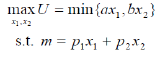
This example uses a quasilinear utility function, \(U = x_1^{\frac{1}{2}} + x_2\). The budget constraint is \(140 = 2x_1 + 10x_2\).
We begin with the analytical approach. We rewrite the constraint and form the Lagrangean, leaving m as a letter (since we want to derive an Engel curve).
We take derivatives and set them equal to zero.
To solve for the optimal values of \(x_1\) and \(x_2\), we follow our usual approach, moving the \(\lambda\) terms over to the right-hand side and dividing the two equations to cancel the \(\lambda\)s.
Notice that the MRS is a function of \(x_1\) alone. This is a property of the quasilinear utility function. We can solve for \(x_1 \mbox{*}\) from the MRS equal to the price ratio equation.
Next, we plug this value into the third first-order condition and solve for \(x_2 \mbox{*}\).
To compute an own units response in \(x_1 \mbox{*}\) given a change in m, we can simply take the derivative with respect to m, which is zero (because m does not appear in the \(x_1 \mbox{*}\) reduced form). Thus, increases in income leave \(x_1 \mbox{*}\) unchanged. In other words, the Engel curve for good 1 is horizontal at 6.25.
The own units response for \(x_2 \mbox{*}\) is \(\frac{dx_2 \mbox{*}}{dm}\frac{m}{x_2 \mbox{*}} = \frac{1}{10}\). This means that an additional dollar in income leads to a \(\frac{1}{10}\) increase in good 2.
We can use the income elasticity formula, \(\frac{dx_1 \mbox{*}}{dm}\frac{m}{x_1 \mbox{*}}\), to compute the income elasticity. At m = 140, the income elasticity of \(x_1 \mbox{*}\) = (0)(140/6.25) = 0, which is perfectly inelastic. This means that changes in m have no effect at all on \(x_1 \mbox{*}\).
These results seem a little strange. Perhaps the numerical approach and Excel can shed some light on what’s going on here.
STEP Open the Excel workbook EngelCurvesPractice.xls, read the Intro sheet, then go to the QuasilinearChoice sheet. It shows the optimal solution, 6.25, 12.75, for m = 140. Change income to 160.
As expected the budget line shifts out.
STEP Run Solver to find the new initial solution. The resulting chart looks like Figure 4.7.
Figure 4.7: Income shock with quasilinear preferences.
Figure 4.7 and your screen show that the value of \(x_1 \mbox{*}\) remained unchanged as income rose from $140 to $160. This consumer maximizes utility by using all of the extra $20 in income on good 2.
Figure 4.7 also displays a key property of the quasilinear functional form: the indifference curves are vertically shifted and actually parallel to each other. Thus, when we increase income, the new point of tangency is found directly, vertically up from the original solution.
STEP Return income to its initial value of $140. Run the Comparative Statics Wizard, applying 5 shocks to income in $10 dollar increments.
Your results should look like the CS1 sheet.
STEP Create Engel and income consumption curves. For the Engel curves, this requires making a chart of \(x_1 \mbox{*}\) as a function of m and another chart of \(x_2 \mbox{*}\) as a function of m. For the income consumption curve, the chart is \(x_2 \mbox{*}\) as a function of \(x_1 \mbox{*}\). Each point on this chart is a point of tangency between the budget line and maximum attainable indifference curve.
Your first attempt at making a chart of \(x_1 \mbox{*}\) as a function of m will not yield a horizontal line at 6.25. Look closely, however, at the y axis scale. The problem is that Solver is reporting numbers very close to, but not exactly, 6.25 as income changes.
But these slight differences in optimal \(x_1\) are not meaningful. They are Solver noise. In fact, for all of these values of m, optimal \(x_1\) really is exactly 25. We need to clean up Solver’s results.
Simply changing the display to fewer decimals will not work. This will change the display of the y axis, but Excel will still have the same number in its memory. Instead, we have to use Excel’s ROUND function to change the numbers produced by Solver.
The ROUND function has two arguments, the cell you want to round and the number of decimal places. So, ROUND(123.456,1) evaluates to 123.5.
STEP Enter this formula in a blank cell, "=ROUND(123.456,-2)" to see what a negative argument does.
We can use the ROUND function to round Solver’s results to the hundredths place. Cell F12 shows how this strategy is implemented.
STEP Apply Excel’s Round function to your comparative statics results and then make a chart of the Engel curve for good 1 using the rounded data. Your final chart should look like the one in the CS1 sheet.
Finally, we can use the CSWiz results to examine the responsiveness of the endogenous variables to the changes in income we applied.
STEP Compute the response to the income changes in own units and income elasticities for \(x_1 \mbox{*}\) and \(x_1 \mbox{*}\). Check your work with the results in the CS1 sheet.
Notice that the responsiveness results from the numerical method are the same as that via the analytical approach.
Perfect Complements
STEP Proceed to the PerfCompChoice sheet to practice on another utility function. This function reflects preferences in which the two goods are perfect complements. This gives L-shaped indifference curves, but our analysis proceeds as usual.
The problem is to maximize the perfect complements utility function subject to the budget constraint. The PerfCompChoice sheet shows that \(p_1 = 2, p_2 = 10, a = b = 1.\)
We do the problem first via the analytical method, leaving m as a letter so we can find \(x_1 \mbox{*} = f(m)\) and \(x_2 \mbox{*} = f(m)\)these are Engel curves for goods 1 and 2.
In section 3.2, we showed how to solve this problem by finding the intersection of two lines on which the solution must lie. Since \(a = b = 1\), the optimal solution must be where \(x_1 = x_2\) (a ray from the origin with slope \(+ 1\)). Of course, the solution must also lie on the budget line, so we can solve this system of two equations and two unknowns by substituting in \(x_1\) for \(x_2\) in the budget constraint equation.
Since \(x_2\) must equal \(x_1\) at the optimal solution, we know \(x_2 \mbox{*} = \frac{m}{12}\).
To compute an own units response in \(x_1 \mbox{*}\) given a change in income, we can simply take the derivative with respect to m, which is simply \(\frac{1}{12}\). This slope is constant and the Engel curve is linear.
The income elasticity at a given value of m can be computed via the point elasticity formula, \(\frac{dx_1 \mbox{*}}{dm}\frac{m}{x_1 \mbox{*}}\). At \(m = 50\), the income elasticity of \(x_1 \mbox{*} = \frac{1}{12}\frac{50}{4.167} = 1\). This means that a 1% change in m will result in a 1% change in \(x_1 \mbox{*}\).
STEP Run the Comparative Statics Wizard on the PerfCompChoice sheet (you can make the change in income $10) and create Engel and income consumption curves.
STEP Compute the response to the income changes in own units and income elasticities for \(x_1 \mbox{*}\) and \(x_2 \mbox{*}\).
Check your work with the results in the CS2 sheet. Notice that the results in Excel are the same as the analytical approach.
The Utility Function Determines the Shape of the Engel Curve
This section ran a comparative statics analysis of a change in income on quasilinear and perfect complement utility functions. This enabled practice in deriving Engel curves and income consumption curves, along with computing responsiveness in own units and elasticities.
The quasilinear function has the peculiar result that the income elasticity of \(x_1 \mbox{*}\) is zero. This happens because the indifference map of a quasilinear utility function is a series of vertically parallel curves. Thus, when the budget line shifts out, the new optimal solution is found directly above the initial solution and \(x_1 \mbox{*}\) remains unchanged.
With the perfect complements utility function, we were able to find an analytical solution even though we could not use the Lagrangean method. The Engel curve for \(x_1 \mbox{*}\) has a constant slope and a unit income elasticity. These are the same properties for the Engel curve we found in the previous chapter using the Cobb-Douglas functional form.
The shape of the Engel curve, its slope and income elasticity are all influenced by the consumer’s utility function. The relationship is complicated, so there is no rule or simple statement about how the functional form of utility determines the Engel curve.
Ernst Engel wanted to know how spending on food changed as income rose. He believed food purchases would increase at a decreasing rate as income increased, as shown in Figure 4.8. This makes common sense. As you get richer and richer, you can buy a much nicer house and cars, but it is difficult to spend a lot more on food. This is known as Engel’s Law.
Figure 4.8: Engel’s Law.
None of three utility functions we have encountered thus far (Cobb-Douglas, quasilinear, and perfect complements) are capable of generating an Engel curve that conforms to Engel’s Law for food purchases. If we were interested in food, we would have to find and use a utility function with an Engel curve that conformed to Engel’s Law. Such functions exist, but as you can imagine, they are more complicated than the computationally simple functions we have used thus far.
Exercises
In the QuasilinearChoice sheet, copy cell B11 and paste it in cell C11. Set income to $200 and run Solver to find the new optimal solution. In cell D11, enter a formula to find the difference between cell C11 and B11. Is this tiny difference meaningful? Explain.
Having changed income and run Solver in question 1, if you connected the initial and new solutions on the chart, you would get a vertical line. Why is this happening? Will this happen with every consumer?
Having changed income and run Solver in question 1, is good 1 a normal or an inferior good? Explain.
Use Word's Equation Editor to solve the general version of the perfect complements problem. In other words, find \(x_1*\) and \(x_2*\) for
References
The epigraph is from pages 487 and 488 of Kenneth E. Boulding, “In Defense of Statics,” The Quarterly Journal of Economics, Vol. 69, No. 4 (November, 1955), pp. 485–502 (www.jstor.org/stable/1881991). As you can tell from the quotation, Boulding had a well-deserved reputation for witty, biting comments. His defense of comparative statics in the article just cited notwithstanding, he once quipped, “Mathematics brought rigor to Economics. Unfortunately, it also brought mortis.”


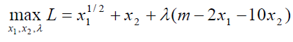
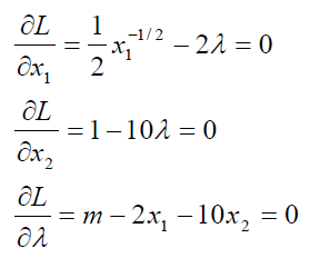
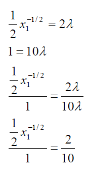
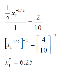
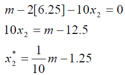
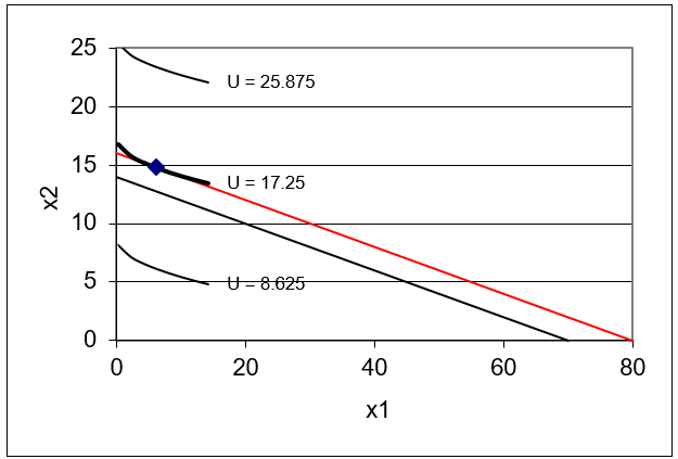 Figure 4.7: Income shock with quasilinear preferences.
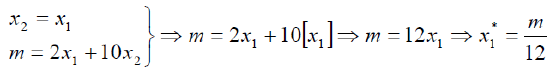
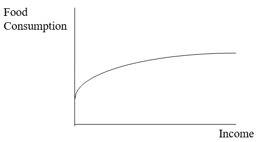 Figure 4.8: Engel’s Law.