This chapter uses a quasilinear utility function to provide practice working with income and substitution effects. There is a surprising twist when using the quasilinear functional form. See how fast you can figure it out.
STEP Open the Excel workbook IncSubEffectsPractice.xls, read the Intro sheet, then go to the OptimalChoice sheet.
Notice that the absolute value of the MRS is less than the price ratio. Because the slope of indifference curve at 16.25,10.75 is less than the slope of the budget constraint, we know the consumer should travel northwest along the budget constraint, buying more \(x_2\) and less \(x_1\), until the MRS \(= \frac{p_1}{p_2}\).
STEP Run Solver to find the initial optimal solution. Figure 4.24 shows this result.
Figure 4.24: Initial optimal solution.
Source: IncSubEffectsPractice.xls!OptimalChoice
STEP Proceed to the CS1 sheet. It shows a comparative statics analysis of an increase in the price of good 1 from $2/unit to $7/unit in $1 increments. It also charts the results as an inverse demand curve for \(x_1\).
The demand curve tracks the total effect of a price change. When the price of good 1 rises from $2 to $3, the quantity demanded falls from \(6 \frac{1}{4}\) to \(2 \frac{7}{9}\). By subtracting the new from the initial value, we see that the total effect is a decrease of \(3 \frac{17}{36}\) units of \(x_1\), displayed in cell F13 as \(-3.47222\).
Income and substitution effects explain how this total effect came to be by dismantling the total effect into two parts that add up to the total.
The substitution effect tells us how much less the consumer would have purchased when price rises strictly from the fact that the relative prices of the two goods have changed. We compute how much income we have to give the consumer to cancel out the reduced purchasing power caused by the price increase to focus exclusively on the relative price change. The substitution effect is always negative.
Figure 4.25 shows a typical decomposition of the total effect (TE) into the substitution effect (SE) and income effect (IE) with indifference curves suppressed to highlight the budget lines under consideration.
Figure 4.25: Typical TE, SE, and IE with \(p_1\) increase.
From point A, price rose and the consumer will now be at point C on the new budget line (labeled \(p_1 \uparrow\)). The dashed line is the result of a hypothetical scenario in which the consumer has been given enough income to purchase the initial bundle A. Notice how the original budget line and the dashed line go through point A. The dashed line has a higher price, but also a higher income. Thus, the movement from point A to point B reflects solely the different relative prices in the goods, without any change in purchasing power. This is the substitution effect.
While the substitution effect is focused on relative prices, the income effect is that part of the response in quantity demanded when price changes that is due to changed purchasing power. From point B, a decrease in income from the dashed to the new budget line leads to a decrease in \(x_1\) (at point C). Thus, \(x_1\) is a normal good from point B to C in Figure 4.25 and the two effects are working in tandem. The demand curve is guaranteed to be downward sloping for this price change.
In the CS1 sheet, we have seen that the demand curve is downward sloping because quantity demanded falls when price rises. But an open question still remains: Do the income and substitution effects work as in Figure 4.25?
We know point A, the initial optimal solution, is \(x_1 \mbox{*} = 6.25\) when \(p_1\) = $2/unit and point C is about 2.78 units of \(x_1\) when price rises to $3/unit. We need point B to do the income and substitution effects analysis.
The first step in finding point B is to use the Income Adjuster Equation to compute how much income to give the consumer in order to cancel out the effect of the reduced purchasing power. \[\Delta m = x_1 \mbox{*}\Delta p_1\] \[\Delta m = [6.25][+1]\]
STEP On the OptimalChoice sheet, set cell B16 to 3.
The chart updates, showing the new budget constraint in red (swinging in since price rose) and the dashed line. To find point B, we need the optimal solution for the dashed line constraint so we need to change in income on the sheet.
STEP Set cell B18 to 146.25. This applies the dashed line budget constraint to this problem. Run Solver to find point B.
Your result might surprise you. Solver says the optimal solution is about 2.78 for \(x_1\), but that is the same answer we had for point C. What is going on here?
We turn to analytical work to shed light on this mysterious result. Following the procedure in section 3.2, we found this reduced form solution for the quasilinear utility function, \(U = x_1^c + x_2\): \[x_1 \mbox{*} = (\frac{p_1}{cp_2})^\frac{1}{c-1}\] We use the initial values of c and \(p_2\) in the OptimalChoice sheet to simplify things a bit: \[x_1 \mbox{*} = (\frac{p_1}{[0.5][10]})^\frac{1}{[0.5]-1} = (\frac{p_1}{5})^\frac{1}{-0.5} = (\frac{p_1}{5})^{-2} = (\frac{5}{p_1})^2 = \frac{25}{p_1^2}\] This is the same kind of expression, \(x_1 \mbox{*} = f(p_1, m)\), that we used in the previous section for a Cobb-Douglas utility function, \(x_1 \mbox{*} = \frac{m}{2p_1}\), to find points A, B, and C.
You might be puzzled. Exactly where is m for the quasilinear reduced form expression for \(x_1\)? It is not there, although a mathematician might say that we could easily include it by writing the reduced form expression like this: \[x_1 \mbox{*} = \frac{25}{p_1^2} + 0m\] The fact that m does not affect optimal \(x_1\) for a quasilinear utility function is the source of the surprising result for point B. We can apply the usual procedure for finding points A, B, and C with a reduced form expression to show this.
Point A is the initial optimal \(x_1\) solution so we plug in \(p_1 = 2\) and find \(x_1 \mbox{*} = \frac{25}{2^2} = 6.25\).
Point C is the new optimal \(x_1\) solution so we plug in \(p_1 = 3\) and find \(x_1 \mbox{*} = \frac{25}{3^2} = \frac{25}{9} = 2 \frac{7}{9}\).
Point B is found using new \(p_1\) and adjusted m, $146.25. But notice that adjusted m is irrelevant because it does not affect \(x_1\). Point B is \(x_1 \mbox{*} = 2 \frac{7}{9}\), the same as point C.
Figure 4.26 shows what is going on here. Unlike the typical case, there is no income effect at all with quasilinear utility, so TE = SE. As usual, the substitution effect is the move from point A to B and the income effect is the movement from B to C. The IE is zero because C is directly below B. The total effect is A to C.
Figure 4.26: TE, SE, and IE with quasilinear utility.
It is the utility function that is driving this result. A utility function with the functional form \(U = f(x_1) + x2\) has no income effect because the indifference curves are vertically parallel. If you shift the budget line via an income shock, the new tangency point will be directly above or below the initial point. In other words, the income consumption curve is vertical. Thus, the total effect is composed entirely of the substitution effect. This is the curious twist produced by the quasilinear functional form.
We saw that the income consumption curve is vertical and Engel curve is horizontal in section 4.2 (see Figure 4.7). Economics is certainly cumulative and ideas learned are often worth remembering because they tend to show up again.
Finally, notice that we now know that quasilinear preferences cannot yield Giffen behavior. After all, if the substitution effect is always negative and the income effect is zero, there is no way for the total effect to ever be positive.
Quasilinear Preferences Yield Zero Income Effects
Splitting a total effect into income and substitution effects works for any utility function. After finding the total effect, the Income Adjuster Equation can be used to determine the income needed to cancel out the change in purchasing power from the price change (i.e., setting the imaginary, dashed budget line). Finding the optimal solution with the new price and adjusted income budget constraint determines point B and allows us to split the total effect in two parts.
Of course, the component parts, SE and IE, need not be equal nor share the same sign. We know that Giffen goods arise when the income effect opposes and swamps the always negative substitution effect.
In the case of quasilinear preferences, we have a situation where there is no income effect. The Slutsky decomposition still applies, however, with the total effect being entirely composed of the substitution effect.
Exercises
Click the button on the OptimalChoice sheet and apply a price decrease for good 1 from $2/unit to $1.90/unit. Compute the total, substitution, and income effects. Show your work.
Use Word’s Drawing Tools to draw a graph similar to Figure 4.26 that shows the total, substitution, and income effects from the 10 cent decrease in price from question 1.
Questions 3 and 4 are difficult. Revisit questions 2 and 3 in EngelCurvesPracticeA.doc (in the Answers folder in the MicroExcel archive) for more detail on the corner solution for this utility function at low levels of income.
With quasilinear utility, the income consumption curve is vertical and the Engel curve horizontal only above a threshold income level. At very low levels of income, we get a corner solution. Click the button on the OptimalChoice sheet and set income to 10. This will generate a corner solution. Compute the total, substitution and income effects from a 10 cent price increase in good 1 (from 2 to 2.1). Show your work.
Use Word’s Drawing Tools to draw a graph depicting your results for question 3.
References
The epigraph comes from page 19 of the second edition of Value and Capital: An Inquiry into Some Fundamental Principles of Economic Theory by John R. Hicks. This remarkable book was explicitly cited in the press release announcing that Hicks had won the Nobel Prize in Economic Science in 1972 (with Kenneth Arrow). "In his most well-known work, the monograph, Value and Capital, published in 1939, Hicks abandoned this [formal] tradition and gave the [general equilibrium] theory an increased economic relevance." See www.nobelprize.org/prizes/economic-sciences/1972/press-release/.
As mentioned in the previous section, the history of income and substitution effects is complicated. Hicks (and Allen) figured out that the total effect could be decomposed into income and substitution effects in the 1930s, two decades after Slutsky’s work. Once Slutsky was rediscovered, Hicks and Allen gave him credit and made the economics profession aware of his contribution. Hicks wrote in Value and Capital that “The present volume is the first systematic exploration of the territory which Slutsky opened up” (p. 19).


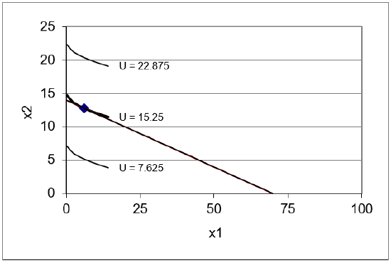
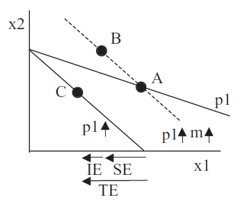 Figure 4.25: Typical TE, SE, and IE with
 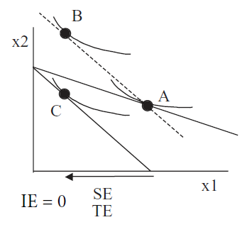 Figure 4.26: TE, SE, and IE with quasilinear utility.
 button on the OptimalChoice sheet and apply a price decrease for good 1 from $2/unit to $1.90/unit. Compute the total, substitution, and income effects. Show your work.
 button on the OptimalChoice sheet and set income to 10. This will generate a corner solution. Compute the total, substitution and income effects from a 10 cent price increase in good 1 (from 2 to 2.1). Show your work.