13.2: Deriving Demand for Labor

A profit-maximizing firm with Cobb-Douglas technology and given prices in all markets (P, w, and r) in the short run can be modeled as solving the following optimization problem: \[\max\limits_{L} \pi = PA\bar{K}^\alpha L^\beta - wL-r\bar{K})\] The previous section found the initial solution for this problem. This section is devoted to comparative statics analysis. How will this firm respond to a change in one of its exogenous variables, ceteris paribus?

Although there are several exogenous variables from which to choose, the responsiveness of optimal L to a change in the wage is of utmost importance. This comparative statics analysis will give us the short run demand for labor.

After deriving the demand for labor in the short run, we will examine the long run demand for labor. A comparison of short and long run wage elasticities of labor reveals that labor demand is more responsive in the long run. We then explore how changes in P affect \(L \mbox{*}\).

Demand for Labor in the Short Run

We begin with numerical methods for a comparative statics analysis of a change in the wage (also called the wage rate is measured in $/hr).

STEP Open the Excel workbook DerivingDemandL.xls and read the Intro sheet, then go to the OneVar sheet.

The layout is the same as the InputProfitMax.xls workbook in the previous section. It is clear from the graphs and the equivalence of wage and MRP below the graphs that the firm is at its optimal solution. The yellow-backgrounded cell, the wage rate, is the shock variable on which we will focus.

STEP Change the wage in the OneVar sheet to $19/hr from the initial value of $20/hr.

It is difficult to see anything in the top graph, however, the isoprofit line is no longer tangent to the TRP. The bottom graph clearly shows that the red diamond (at L = 1431 hours) has a marginal revenue product greater than the marginal factor cost (equal to the wage). Cells H40 and I40 show that the wage is less than MRP.

STEP Since the firm is no longer optimizing, run Solver to find the new optimal solution.

You will find that, to maximize profits, the firm will hire 1757 hours when the wage falls to $19/hr, ceteris paribus. At this level of labor use, the marginal revenue product once again equals the marginal factor cost.

Although we have only two data points, it should be clear that the firm will hire that amount of labor where the marginal revenue product equals the wage, in the short run. This means that the marginal revenue product curve is the firm’s (inverse) demand for labor curve. Quote the firm a wage and it will look to its MRP curve to decide how much labor to hire.

We have two points on the demand for labor curve; at w = $20/hr, \(L \mbox{*}\) = 1431 hours and at w = $19/hr, \(L \mbox{*}\) = 1757 hours. Can we pick more points off of the demand for labor curve?

STEP Set the initial wage back to $20/hr and use the Comparative Statics Wizard to apply five $1/hr decreases in the wage. Create charts of the demand for labor and the inverse demand for labor.

Your results should look like those in the CS1 sheet. The CSWiz output makes common sense. As the wage drops, the firm hires more labor. Look also at the objective functionas wage falls, maximum profits are rising. The key idea here is that firm hiring decisions are driven by profit maximization. The reason why L increases as w falls is that this response is profit maximizing.

Like demand curves in the Theory of Consumer Behavior, the pricethe wage in this casecan be placed on the x or y axis. The two displays use the same information and convey the same message.

We can also derive the short run demand for labor via analytical methods. This problem was presented in the previous section. For your convenience, it is repeated below.

We need to leave w as a variable, but for maximum generality we solve for \(L \mbox{*}\) as a function of all parameters.

\[\max\limits_{L} \pi = PA\bar{K}^\alpha L^\beta - wL-r\bar{K})\] We take the derivative with respect to L, set it equal to zero, and solve for \(L \mbox{*}\).

This expression is the demand curve for labor. If we substitute in values for all exogenous variables except w, we can plot \(L \mbox{*}\) as a function of w, ceteris paribus.

Do the numerical methods based on the CSWiz add-in agree with the analytical derivation of the demand for labor?

STEP In the CS1 sheet, click on cell C16. This is Solver’s answer for \(L \mbox{*}\) when the wage is $20/hr.

Do not be misled by all of the decimal places. That is false precision.

STEP Click on cell E26. It displays \(L \mbox{*}\) when the wage is $20/hr based on the reduced-form solution.

Do not be misled by the number displayed in cell E26. This is Excel’s display for the formula entered into that cell. Excel’s memory has a different number.

STEP Widen column E to see more decimal places.

We proceed slowly because things can get confusing here. Consider this hierarchy of truth:

1. Solver is giving a number close to the exact right answer in cell C16.
2. Excel is representing the exact right answer as a decimal in cell E26.
3. The exact right answer is \(\frac{w}{\beta PA\bar{K}^\alpha}^{\frac{1}{\beta -1}}\) evaluated at w = $20/hr, along with the other parameter values.

STEP To see that E26 is not the exact answer, make column E very wide, then select cell E26 and click Excel’s Increase Decimal button repeatedly.

You will see that, eventually, Excel will start reporting zeroes. Excel has finite memory and, therefore, it cannot compute an infinite number of decimal places for the exact answer. The decimal representation of the exact answer stored in Excel’s memory is not the exact answer.

To be clear, Excel can display the exact answer if it is an integer or fraction that can be represented with finite memory. For example, \(\frac{x}{7}\), evaluated at \(x=14\) is 2 so, no problem for Excel. If 2 is the answer, Excel has it exactly right. Evaluating at \(x=1\) means there is no decimal representation with a finite number of digits. Excel cannot display the exact answer in this case. Enter \(=1/7\) in a cell, widen the column, and click the Increase Decimal button repeatedly to see that Excel eventually starts showing zeroes.

Thus, neither E26 nor C16 is the exact answer. They are both so close to the answer, however, that we can say they "substantially agree" and are correct.

We can also use the analytical approach to reinforce the idea that the short-run (inverse) demand for labor is the marginal revenue product of labor.

The first-order condition gives the equimarginal rule. \[\begin{gathered} %star suppresses line # \frac{d \pi}{dL} = \beta PA\bar{K}^\alpha L^{\beta-1} = w\end{gathered}\] The term on the left is the MRP. Evaluating the \(\beta PA\bar{K}^\alpha\) portion at their initial values gives 123.0187 (as shown in cell K26 of the CS1 sheet). Thus, \(MRP=123.0187L^{\beta-1}\) and at \(\beta = 0.75\), \(MRP=123.0187L^{0.25}\).

The CS1 sheet has an inverse demand for labor chart. Is the relationship in this chart the same as the MRP function that we just found? Let’s find out. By finding the function that fits the data in the inverse demand for labor chart, we can compare this relationship to the MRP function.

STEP Right-click on the series in the inverse demand for labor chart and select the Add Trendline option. Select the Power fit, scroll down and check the Display equation on chart option. Click OK. Move the equation (if needed) and increase the font size to see it better. Scroll right to see what your chart should look like.

The answer is clear: The fitted curve that reveals the function for the inverse demand curve for labor is the marginal revenue product of labor curve. The fitted curve’s coefficient and exponent are almost exactly that of the MRP.

Next, we turn our attention to the wage elasticity of labor demand. We can compute the elasticity at a point or from one point to another. We do the former below and leave the latter as an exercise question.

Elasticity at a point begins by finding the derivative of the reduced-form expression. We substitute in the known value for \(\beta PA\bar{K}^\alpha=123.0187\) in the denominator and \(\beta =0.75\) in the exponent. \[\begin{gathered} %star suppresses line # L \mbox{*}=(\frac{w}{\beta PA\bar{K}^\alpha})^{\frac{1}{\beta-1}}= (\frac{w}{123.0187})^{\frac{1}{0.75-1}}=(\frac{w}{123.0187})^{-4}\end{gathered}\] To take the derivative with respect to w, we isolate w. \[\begin{gathered} %star suppresses line # L \mbox{*}=(\frac{w}{123.0187})^{-4}=\frac{w^{-4}}{123.0187^{-4}}=(\frac{1}{123.0187^{-4}})w^{-4}\end{gathered}\] Now we can apply our usual derivative rule, moving the exponent to the front and subtracting one from it. \[\begin{gathered} %star suppresses line # \frac{dL \mbox{*}}{dw}=-4(\frac{1}{123.0187^{-4}})w^{-5}\end{gathered}\] This expression is merely the slope or instantaneous rate of change of optimal labor hired as a function of the wage. To find the elasticity, we must multiply the derivative by the ratio w/L. \[\begin{gathered} %star suppresses line # \frac{dL \mbox{*}}{dw}\frac{w}{L}=-4(\frac{1}{123.0187^{-4}})w^{-5}\frac{w}{L}\end{gathered}\] But we have an expression for L, so we substitute it in. \[\begin{gathered} %star suppresses line # \frac{dL \mbox{*}}{dw}\frac{w}{L}=-4(\frac{1}{123.0187^{-4}})w^{-5}\frac{w}{(\frac{1}{123.0187^{-4}})w^{-4}}\end{gathered}\] The \(123.0187^{-4}\) terms cancel. And \(w^{-5}\) times w in the numerator is \(w^{-4}\) so that cancels with \(w^{-4}\) in the denominator. We are left with this. \[\frac{dL \mbox{*}}{dw}\frac{w}{L}=-4\] As has happened before (remember the price and income and cross price elasticity of demand?), the Cobb-Douglas functional form produces a constant wage elasticity of short run labor demand.

This elasticity value says that labor demand is extremely responsive to changes in the wage. We would not expect to find such a large wage elasticity of short-run labor demand in the real world. For a Cobb-Douglas production function, the elasticity is driven by the value of beta. If we had left \(\beta\) in the expression for optimal L instead of using 0.75 (see the first two exercise questions), we would get this expression for the wage elasticity of labor demand: \[\frac{dL \mbox{*}}{dw}\frac{w}{L}=\frac{1}{\beta-1}\] If we compute the elasticity from one point to another, say from a wage of $20/hr to $19/hour (see exercise question 3), we will get a different answer than \(-4\). That makes sense since we know that \(L \mbox{*}\) is non linear in w. As the change in the wage approaches zero, the elasticity computed from one point to another approaches \(-4\).

Demand for Labor in the Long Run

If we relax the assumption that capital is fixed, we change the firm’s planning horizon from short to long run. The TwoVar sheet implements the firm’s long run input profit maximization problem. There are two endogenous variables, labor and capital, and no fixed factors of production.

STEP To derive the firm’s long run demand for labor, use the Comparative Statics Wizard from the TwoVar sheet. As you did in the short run analysis, apply $1 decreases in the wage.

Your results should show labor use rising as wage falls, just as in the short run. But what about the elasticityis it the same in the short and long run?

STEP Use your CSWiz results to compute the wage elasticity of labor demand from a wage of $20/hr to $19/hr. Is it close to \(-4\), the point elasticity at w=$20/hr?

The CSCompared sheet is similar, but not the same as your results. It shocks wage by $1/hr increments in the short and long run.

The difference in the elasticity is dramaticlabor demand is incredibly responsive in the long compared to the short run. The elasticity almost triples, from \(-3.5\) to almost \(-11\). You should find the same result with your CSWiz data for a wage decreasethe long run elasticity is much higher (in absolute value) than in the short run. What is going on?

Figure 13.4 provides an answer to this question. The movement from point A to B is the short run response for a $1/hr wage increase. As the short run results in the CSCompared sheet show, when the wage rises from $20/hr to $21/hr, \(L \mbox{*}\) falls from roughly 1,431 hours to 1,178 hours.

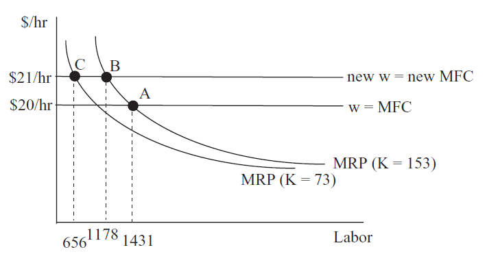Figure 13.4: Why \(L \mbox{*}\) is more responsive to \(\Delta\)w in the long than short run.

In the short run, capital stays fixed and the firm moves along its marginal revenue product curve (which as we already know is the firm’s short run demand for labor) as the wage changes. The \(K=153\) in the parentheses signals that this is the value of K for this MRP schedule.

In the long run, however, the adjustment is different. The data in the CSCompared sheet show clearly that the firm will change both labor and capital as the wage rises. Notice that capital falls from 153 machines to 73 machines as the wage rises from $20/hr to $21/hr.

This change in capital shifts labor’s marginal revenue product curve. As shown in Figure 13.4, the firm’s long run response to the change in the wage is from A to C, not simply A to B. It decreases labor use as it moves along the initial MRP and then again when MRP shifts as K falls. This is the reason why the wage elasticity of labor demand is more responsive in the long run.

Figure 13.5 shows the firm’s long run demand for labor and that it is no longer the MRP curve. Because capital falls as wage rises, leading to a further decrease in labor hired, the firm is much more responsive to changes in the wage.

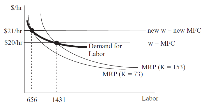Figure 13.5: The long run demand for labor.

It is clear that the inverse labor demand curve shown in Figure 13.4 is flatter in the long run than the MRP curve (which is the short run inverse demand for labor). A wage decrease would stimulate more labor hired in the long than short run because K would rise in the long run.

The Shutdown Rule and the Demand Curve for Labor

Recall that, on the output side, the supply curve is the MC curve when \(P > AVC\).If \(P < AVC\) where \(MR = MC\), then the firm ignores this marginal signal (which is the top of a local profit hill) and shuts down (\(q = 0\)). The supply curve has a tail where the quantity supplied is zero when the price falls below average variable cost.

There is a similar tail, with \(L=0\), on the demand curve for labor. The previous section showed that if \(w>ARP\), the firm will shut down, hiring no labor and producing no output.

STEP Proceed to the Graphs sheet to quickly review this concept. Use the pull down menu to change the firm’s output price and place the firm in any of the four profit positions. Select Neg Profits, Shutdown to see that the firm will shut down when P is so low that it shifts ARP down so much that \(w>ARP\). This is analogous to the \(P < AVC\) Shutdown Rule.

The Shutdown Rule means that we have to change our definition of the demand curve for labor to get it exactly right. In the short run, the inverse demand curve is the MRP curve, as long as \(w> ARP\); otherwise it is zero, as shown in Figure 13.6.

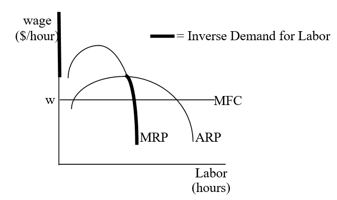Figure 13.6: The short run inverse demand for labor.

The Shutdown Rule is usually presented from the output side as \(P < AVC\). This version of the rule is perfectly compatible with the input side version of the shutdown rule, \(w>ARPL\). Either wage increases or output price decreases can trigger a shutdown.

In Figure 13.6, it is easy to see what is happening when wage increasesthe horizontal MFC line shifts up and it rises above ARP, the firm shuts down. What is happening on the output side? Remember that as wage rises, cost curves on the output side shift up. At the precise point at which a higher wage triggers the decision to not hire any labor, the AVC curve will have shifted above P and the firm will decide to not produce any output.

The same story is at work when P falls. On the output side, it easy to see that when the horizontal \(P=MR\) line falls below AVC, the firm shuts down. What is happening on the input side? As P falls, the MRP and ARP curves in Figure 13.6 shift down. At the precise moment when P falls below AVC and the firm decides to produce no output, the ARP shift below the horizontal wage line in Figure 13.6 and the firm will decide to hire no labor.

Demand for Labor Depends on P

Another comparative statics analysis for input profit maximization revolves around the effect that P has on \(L \mbox{*}\). This shows how the demand for labor is a derived demand from the desirability of the product. In other words, the stronger the demand for the product, the greater the demand for labor.

Suppose demand for bread rises in our Excel workbook. This increases P, ceteris paribus. What happens to L? We explain the short run response here and leave the long run for exercise questions 4 and 5.

STEP Return to the OneVar sheet. Return the wage to $20/hr. Run Solver.

Instead of simply changing P and running Solver again, we want to see what effect P has on the graphs that show the initial solution.

STEP Change P to $2.10 and look carefully at the charts.

It is difficult to see that the TRP curve has changed so that it is no longer tangent to the isoprofit line, but the bottom chart clearly shows that the initial solution is no longer optimal. What happened?

From our analytical work, we know that \(MRP = \beta PA\bar{K}^\alpha L^{\beta-1}\) so it is clear that an increase in P will shift the MRP curve up. That is what you are seeing in the bottom graph on the OneVar sheet. Return P to $2/unit to see that MFC stays constant (w remains unchanged), but MRP is moving.

STEP With P=$2.10, run Solver. What happens to \(L \mbox{*}\)?

Not surprisingly, the firm wants to hire more labor. The reason is that the MRP curve shifts and a new solution is found where the new \(MRP = w\). Labor cost and productivity are unchanged, but the demand for labor is affected by consumer’s desire for the product (expressed through the P). We say that that demand for labor is a derived demandthe firm’s need for labor (and other inputs) comes from the fact that it has customers who want its product.

Figure 13.7 shows what happens as you increase the product price. If the demand for a firm’s output is high, the price will be high, and this will induce an increased demand (shift) for labor.

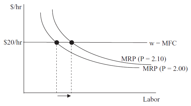Figure 13.7: Demand for L is a derived demand.

It is easy to see that labor is a derived demand by considering professional sports. Pro athletes in major sports make a lot of money because they are in high demand. Sports teams know that the price of the good they produce (including broadcast and streaming revenue) is high. The output side is most definitely reflected in the input side via the product price.

Marginal Productivity Theory of Distribution

The input side profit maximization problem can be used to examine the distribution of firm revenues. The basic idea is that shares are a function of an input’s productivity: The more productive the input, the greater its share.

STEP From the TwoVar sheet, run a comparative statics experiment that changes the exponent on labor from 0.75 to 0.755 (5 shocks of 0.001). In the endogenous variables input box, be sure to track not only L and K, but also the shares received in cells C44:C46.

Check your results with the CS3 sheet. The CS2 sheet has the outcome of a change in alpha, the exponent on capital. It explains how "large" shocks of, say, 0.1 will cause catastrophic failure as \(\alpha + \beta\) approaches \(+1\). This is why the change in beta so smallto stay away from the singularity.

By increasing the exponent on labor in the Cobb-Douglas production function, labor’s productivity rises. In other words, labor can make more output, ceteris paribus, as the exponent on labor increases. The firm maximizes profit by using more labor and labor’s share of firm revenues rises.

The CSWiz data show that we can immediately determine the percentage share of revenues gained by each input by the input’s exponent in the production function. Although a different production function may not have this simple short-cut to determine the percentage share of revenues accruing to each input, it remains true that an input’s share will depend on its marginal productivity.

Whereas algebraic convenience and simplicity are often invoked as a rationale for utilizing the Cobb-Douglas functional form, in the case of factor shares, a strong empirical regularity supports the use \(AK^\alpha L^\beta\). About 2/3 of national income has gone to labor and 1/3 to capital. “In fact, the long-term stability of factor shares has become enshrined as one of the “stylized facts” of growth” (Gollin, 2002, pp. 458–459). More recent measurements of factor shares shows that capital is gaining a greater share and this is an active, exciting area of research.

Labor Demand Highlights

The most important comparative statics exercise on the input side is to derive the demand for inputs. This chapter focused on labor demand and showed that the short run demand for labor is the marginal revenue product of labor curve.

In the long run, however, the demand for labor is not the MRP curve because \(K \mbox{*}\) changes as w changes. For this same reason, labor demand is more responsive to changes in the wage in the long run.

Whether in the long or short run, the demand curve for labor is subject to the same Shutdown Rule qualification as the supply curve for output. If the wage is higher than the ARP at the point at which \(MRP = MFC\), the firm will hire no labor. This coincides perfectly with the firm’s decision to shut down on the output side, producing no output.

In addition to changes in the wage, this chapter explored the effects of a change in product price. As P increases, \(L \mbox{*}\) rises. In terms of the canonical graph, an increase in P shifts the MRP and leads to a new optimal solution. This leads economists to think of and say that labor demand is a derived demand because the price of the product influences how much labor the firm wants.

This section ended by pointing out that an input’s productivity determines its share of firm revenues. As productivity rises, so does the percentage share accruing to that input. Productivity is a key variable in determining input use and distribution of revenues.

Exercises

1. Derive the wage elasticity of short run labor demand for the general case where \(L \mbox{*}=(\frac{w}{\beta PA\bar{K}^\alpha})^{\frac{1}{\beta-1}}\). Show your work, using Word’s Equation Editor.
2. Does your result from the previous question agree with the \(-4\) value obtained in the text?
3. Compute the wage elasticity of short run labor demand (using the parameter values in the OneVar sheet) from w=$20/hr to $19/hr. Show your work.
4. Use the Comparative Statics Wizard to analyze the effect of an increase in the product price in the long run. Compute the P elasticity of \(L \mbox{*}\) from \(P = 2.00\) to \(P 2.10\). Copy and paste your results in a Word document.
5. Is \(L \mbox{*}\) more responsive to changes in P in the short run or long run? Explain why.

References

The epigraph is from page 523 of David S. Landes, The Wealth and Poverty of Nations: Why Some are So Rich and Some So Poor (paperback edition, 1999; originally published, 1998). Landes was an economic historian interested in economic development. He asked really difficult, fascinating questions: "How and why did we get where we are? How did the rich countries get so rich? Why are the poor countries so poor? Why did Europe (‘the West’) take the lead in changing the world?" (p. xxi). His answers are opinionated and clear.

The idea that a profit-maximizing firm will use and reward factors according to productivity has a normative or ethical dimension. John Bates Clark, one of the first well-known American economists, argued in The Distribution of Wealth (1899) that the equimarginal principle was not only efficient, but also fair. Paying factors according to productivity showed that capitalism was just. For more modern reading on morality or ethics in economics, from one end of the spectrum to the other, see Robert Nozick, Anarchy, State, and Utopia (1974) and John Rawls, A Theory of Justice (1971).

You are undoubtedly familiar with the Nobel Prize in Economic Sciences, but the John Bates Clark Medal is given every two years "to that American economist under the age of forty who is adjudged to have made the most significant contribution to economic thought and knowledge." See www.aeaweb.org/about-aea/honors-awards/bates-clark for a complete list of winnersit is peppered with Nobel Prize winners.

In his paper reconciling time series and cross section data, Douglas Gollin, "Getting Income Shares Right," The Journal of Political Economy, Vol. 110, No. 2 (April, 2002), pp. 458–474, www.jstor.org/stable/10.1086/338747, says that Cobb and Douglas "were among the earliest authors to point out that, for the United States, the labor share of income appeared to be roughly constant over time, regardless of changes in factor prices" (pp. 460–461). As mentioned in this section, this remarkable constancy of labor shares has crumbled recently, as labor’s share has fallen. For a more recent review of labor’s share, see conversableeconomist.blogspot.com/2018/02/behind-declining-labor-share-of-income.html.