17.4: Inefficiency of Monopoly

Partial equilibrium analysis is based on the idea that each good and service with resources allocated via the market system has supply and demand curves. Prices signal quantities demanded and supplied and are pushed toward equilibrium by market forces. The equilibrium quantity is the market’s answer to society’s resource allocation problem.

If an omniscient, omnipotent social planner, OOSP, were to maximize the consumers’ and producers’ surplus of an individual good or service, she would explicitly order the production of the socially optimal amount of each good and service.

A critical result from this analysis is that a properly functioning market’s equilibrium quantity equals the socially optimal quantity. This is what we mean when we say that a properly functioning market correctly solves society’s resource allocation problem. There is no deadweight loss because the correct output is produced.

This section focuses on the following question: What happens if one of the goods is produced by a single seller (instead of the many individual firms that define perfect competition)?

In other words, we explore the welfare effects of monopoly. Our analysis is based on partial equilibrium and uses the tools of consumers’ and producers’ surplus. We evaluate monopoly by figuring out what a monopolist would produce, and then compare the monopoly output to the socially optimal output.

STEP Open the Excel workbook MonopolyDWL.xls, read the Intro sheet; then go to the PC sheet.

The linear demand and supply curves have the same parameter values used in previous examples. The equilibrium price is $100, which yields an equilibrium output of 125 units. Because the socially optimal level of production is also 125 units, the market yields an efficient allocation of resources.

Notice that at the socially optimal and competitive market solution, since supply is the sum of firm’s marginal costs, we know that aggregate marginal cost equals demand. This is called marginal cost pricing and is indicative of a socially optimal solution. We will see in a moment that monopoly does not share this property.

The Monopoly Solution

Suppose all of the firms that produce a product in a perfectly competitive market were to merge into a giant, single firm. We assume that the cost structure stays exactly the same. In other words, the supply curve, which was the sum of the individual marginal cost curves, now becomes the monopolist’s marginal cost curve.

Assuming that the costs of many firms would be the same costs faced by a single firm is a stretch. After all, the monopolist needs only one CEO and one customer service hotline. In other words, there are likely to be economies of scale in administration, distribution, and other areas. We assume this away in our comparison of perfect competition and monopoly. The idea is that the only difference is in the impact on the observed output when we have many firms in competition versus a single firm.

The monopolist will behave differently than the many firms did because there is no competition. Unlike the competitive result, where price is determined by the interaction of many buyers and sellers, the monopolist will choose the profit-maximizing price and quantity.

Chapter 15 explained monopoly profit maximization. What is different in this section is that, after determining the output chosen by the monopolist, we want to evaluate it using the tools of partial equilibrium analysis.

Our path is straightforward: we will solve the monopolist’s problem with analytical and numerical methods, then we judge the monopoly outcome.

We know the monopolist will maximize profit by finding that quantity where \(MR = MC\). The former is given by the demand curve, but what about MC?

The MC function is given by the supply curve parameters in the PC sheet. Once a monopoly takes over, it does not have a supply curve, but it does have a marginal cost function, which is the same as the supply curve (because of our assumption that there is no difference in costs between a competitive industry and a monopoly).

Thus \(MC = 35 + 0.52Q\) and we can derive demand from the demand curve, as we have done before: \[TR=P(Q)Q=(350-2Q)Q=350Q-2Q^2\] \[MR=\frac{dTR}{dQ}=350-4Q\] As expected, we see that MR has twice the slope of the demand curve.

To find the monopolist’s optimal Q, we set \(MR = MC\) and solve for \(Q \mbox{*}\): \[350 - 4Q \mbox{*} =35+ 0.52Q\mbox{*}\] \[4.52Q\mbox{*}=315\] \[Q\mbox{*} \approx 69.69\]

To find \(P\mbox{*}\), we use the demand curve to compute the highest price obtainable for that quantity. \[P=350-2Q=350-2[69.69] \approx \$210.62\]

STEP Proceed to the Monopoly sheet to use numerical methods.

The graph has been augmented with the MR curve and the supply curve is now labeled MC. The MR curve was always there, but perfectly competitive firms cannot exploit it.

The sheet shows the monopoly price and output in cells B15 and B16 based on the analytical solution. Before we examine the deadweight loss and surplus information, we confirm that numerical methods agree.

When you run Solver, notice that the Solver dialog box is set up to choose that quantity that sets cell B20 to zero. The initial output of 50 units is too low. The fact that \(MR - MC\) is $89 means that the 50th unit of output adds $89 more in profits and, therefore, more should be produced.

STEP Run Solver to find the Q that sets \(MR - MC\) equal to zero.

After running Solver, you should see that cell B20 equals zero and that the Solver solution agrees (not exactly, but practically speaking) with the analytical method. This is not a surprise.

We now arrive at the key moment. How to judge the monopoly solution?

Evaluating Monopoly

We know the monopolized market will have an optimal output of 69.69 units and a price of $210.62/unit. The evaluation of this outcome is based on computing the consumers’ surplus, CS, and producers’ surplus, PS, generated by the monopoly, and then comparing it to the socially optimal result.

The socially optimal result, at \(Q=125\) units, yields $19,688 of total surplus.

STEP Cell F19 displays $15,625 of consumers’ surplus. Click on the cell to see its formula: = 0.5*(d0_ \(-\) P)*Q. P and Q are named cells for the perfectly competitive solution of 100 and 125, respectively.

Cell F20 has producers’ surplus at \(Q = 125\). Cell F21 adds CS and PS. The total surplus of $19,688 is the maximum surplus possible and it is obtained when 125 units are produced.

Now, consider what happens under monopoly.

STEP Cell I19 shows a dramatic drop in CS. Click on the cell to see its formula: =0.5*(d0_-Pm)*Qm. Pm and Qm are named cells for the monopoly price and output.

The monopolist has lowered output and raised the price, relative to the competitive solution. This has greatly reduced consumer’s surplus.

Cell I20 shows producers’ surplus. It has more than doubled from what it was when the market was competitive. Its formula is: =(Pm-I18)*Qm + 0.5*(I18-s0_)*Qm. The first part of the formula is a rectangle. The height is the monopoly price minus the MR (or MC given that they are equal). The length is the monopoly output. A large part of this rectanglefrom the monopoly price to the perfectly competitive equilibrium priceused to belong to the consumers. It has been taken by the monopolist and helps explain why CS and PS have changed so dramatically.

So, CS has fallen and PS has risen, what is the overall outcome? Cell I21 adds CS and PS under monopoly. The total surplus of $15,833 is lower than the maximum possible surplus of $19,688. The difference, $3,855 (in cell I23), is the lost surplus due to monopoly. This is also known as the deadweight or welfare loss.

STEP Click the button to see a visual presentation in the graph of the deadweight loss of monopoly. It is a Harberger triangle.

Figure 17.17 is a canonical graph in microeconomics. It shows that the monopoly output is too low (so too few resources are allocated to this market) and the deadweight loss or Harberger triangle is used to indicate the inefficiency generated by monopoly.

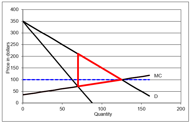
Figure 17.17: The deadweight loss from monopoly.

Source: MonopolyDWL.xls!Monopoly.

Because the monopoly solution does not equal the socially optimal output, we say there is a market failure. It is a failure in the sense that resources are not optimally allocated from society’s point of view.

Inframarginal thinking can be applied to Figure 17.17. The basic idea is that all of the output in the range from the monopoly solution, roughly 70 units, up to the socially optimal output level of 125 units, exhibits unrealized gains from trade. For example, the marginal cost of producing the 100^th unit is \(35 + 0.52x100\), which equals $87. The demand curve tells us that consumers are willing to pay up to $150 for the 100^th unit. Clearly, the 100^th unit should be produced because the additional satisfaction (as measured by willingness to pay) is greater than the additional costs of production.

The monopolist refuses to produce and sell the 100^th unit, however, because of an implicit restriction. Monopoly power allows the firm to set the price, but all units must be sold at the same price. Selling the 100^th unit at a price of $150/unit means that all units must be sold at this price. Doing this would lower monopoly profit.

But the partial equilibrium welfare analysis critique of monopoly does not ride on the fact that monopoly forces consumers to pay higher prices than under a competitive market. The real problem with monopoly is that it produces too little outputit produces less than the socially optimal level. This causes too few resources to be allocated to the production of the monopolized good or service. We measure the amount of this inefficiency in resource allocation by the deadweight loss.

Yet another way to frame the inefficiency of monopoly is to focus on the fact that the monopolist produces where \(MR = MC\) and this differs from \(P = MC\) because MR diverges from the demand curve. A competitive market yields a socially optimal output because output is produced up to the point at which marginal cost equals the price (i.e., marginal cost pricing).

Figure 17.17 makes clear that the monopolist does not conform to marginal cost pricing. \(MR = MC\) yields the output that maximizes profits, but \(P = MC\) (where demand intersects supply or the aggregate marginal cost curve) is the socially optimal output. The monopolist is not interested in social optimality and, therefore, does not obey marginal cost pricing.

Elasticity Rules Again

In the previous section, we saw that the deadweight loss from a quantity tax depended on the price elasticities of supply and demand. The same holds true for monopoly.

STEP Click the button in the Monopoly sheet with red DWL triangle displayed.

Demand is flatter, while going through the same competitive equilibrium point, Q = 125, P = 100. Thus, demand is more elastic at this point.

The button is actually a toggle. By clicking it repeatedly, you can switch back and forth from the original, more inelastic demand (price elasticity of \(-0.4\) at \(P=100\)) to the more elastic demand (price elasticity of \(-0.8\) at \(P=100\)).

STEP Click the D more and less elastic button a few times to convince yourself that the deadweight loss from monopoly is in fact larger when demand is more inelastic.

While cell E17 shows that DWL is higher when demand is more inelastic, we can make a graph that clearly shows this.

STEP Copy the Monopoly sheet and make the elasticity on the copy different than on the original sheet. Copy the chart in one sheet and paste it on top of the chart in the other sheet.

There is no fill in the chart so it is transparent. Your chart should look like Figure 17.18.

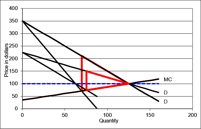Figure 17.18: Comparing deadweight loss with different price elasticities of demand.

In Figure 17.18, the larger red triangle is the deadweight loss of $3,855 in the initial case, with a price elasticity of demand of \(-0.4\) at \(P=100\). The smaller red triangle is DWL with more elastic demand of \(-0.8\). The DWL is lower, falling to $1,870, when demand is more elastic.

Deadweight loss falls when demand is more elastic because the output does not deviate as much from the socially optimal result and the monopoly price is much lower. Hence, the Harberger triangle is both shorter and thinner.

Intuitively, the more inelastic is demand, the greater is the monopoly power. A monopolist who enjoys an extremely inelastic demand is able to charge very high prices and the gap from marginal cost to demand for the inframarginal units will be large. This is the primary reason why the deadweight loss from monopoly increases as demand becomes more inelastic.

This example shows why economists use deadweight loss to measure inefficiency instead of simply the deviation in output from its optimal value. The monopolist does not change output by much when demand is more inelastic (\(-0.4\)), but the fact that consumers are willing to pay a lot more for the inframarginal units drives the large increase in deadweight loss.

Notice that the effect of elasticity on DWL is different than what we obtained for quantity taxes. In that case, more inelastic demand led to lower deadweight loss. The effect is reversed with monopoly, but the principle that elasticity rules remains true.

Monopoly and Price Discrimination

Although we usually assume a monopolist must charge the same price for all units sold, sometimes a seller can charge different prices for the same product. This is known as price discrimination and it enables profits to be even greater than when a single price is charged to all customers.

Charging different prices to see a movie in the afternoon versus the evening, different prices for coach versus first-class on a plane or train, and different net tuition to students (in the form of differing amounts of financial aid) are all examples of price discrimination. In each case, the firm is able to increase its profits by separating consumers into different groups and charging them different prices for the same good or service.

Sometimes firms try to slightly change the product so it isn’t so obvious that the exact same thing is being sold at different prices. Offering first-class payers pre-boarding and free drinks on a plane is an example of this. As is the bigger portions of a dinner versus lunch version of a dish at a restaurant. The difference in prices for the first-class and dinner versions of these products is not grounded in higher costs.

What is really going on here is coming entirely from the demand side. Some consumers are willing to pay more and firms are taking advantage of this.

People can get really upset at price discrimination. Dry cleaners can get in hot water when they charge different prices for cleaning men’s versus women’s clothing that is almost identical. It can be a fun game to spot examples of price discrimination.

There are three requirements for price discrimination to work:

1. Some degree of monopoly power (facing a downward sloping demand curve).
2. The firm must be able to segregate customers into groups (splitting the overall demand curve into subgroup demands).
3. There must be a way to seal the markets to prevent resale from the low-price to the high-price market, which is called arbitrage.

Assuming these requirements are met, we can construct a simple example that illustrates the essential logic of price discrimination. The idea is to separate price sensitive from insensitive consumers and then charge insensitive ones more.

STEP From the Monopoly sheet, click the Reset button and change cell E8 to 0 (zero).

This makes MC constant at $35/unit and makes it easy to find the optimal solution and deadweight loss.

STEP With MC constant at $35/unit, run Solver to find the monopolist’s optimal solution.

Your screen shows that the monopolist will produce 78.75 units of output and charge a price of $192.50. CS under monopoly is $6,202 and PS is $12,403.

STEP Click the 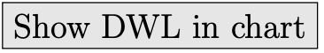button to display the Harberger triangle. Its area is the DWL of $6,202.

The fact that CS equals the DWL is not a coincidence. This is a property of linear demand and constant MC.

Now, suppose that this monopolist can separate the overall market demand, given by the inverse demand function of \(P = 350 - 2Q\), into two separate markets with two subdemands. For example, the two subdemands could be given by \[\text{Market 1: }P = 450 - 6Q\] \[\text{Market 2: }P = 300 - 63Q\] The coefficients in the two separate markets must be consistent with the coefficients in the overall market inverse demand curve. The intercept and slope are not randomly drawn. If the price is zero, quantity demanded in Market 1 is 75 (= 450/6), while Market 2’s quantity demanded would be 100 (= 300/3). The sum of the two is 175, which equals the quantity demanded at \(P = 0\) using the overall inverse demand curve. At \(P = 300\), Market 1’s quantity demanded is 25 and Market 2’s is zero, and this sum equals the quantity demanded using the overall demand curve.

How can a monopolist take advantage of the ability to separate the overall market into two sealed, separate subdemands?

The intuitive answer is simple: Instead of charging the same price, $192.50, to all customers, increase the price in the market with more inelastic demand and reduce it in the other market. The customers in Market 1 can be charged a higher price than those in Market 2. This will lead to greater profits.

We can see a concrete demonstration of this and figure out exactly what prices we should charge in our example.

STEP Proceed to the TwoPriceDisc sheet to see this plan in action.

Unlike the Monopoly sheet, there is no need to run Solver. The analytical solution has been entered and all cells and charts will instantly respond to changes in parameter values.

The top of the sheet shows how a perfectly competitive market would behave if there were two separate markets. Marginal cost pricing would result from competition so both markets would have the same price of $35/unit (cells B11 and B15). Market 2 would produce slightly more (B16) than Market 1 (B12), but the sum of the two (B20) would equal the perfectly competitive output of perfect competition for a single market. Thus, the ability to price discriminate, separating a single market demand into two separate, sealed subdemands, has no effect under perfect competition.

The outcome is different for monopoly. We begin by pointing out that the price elasticity of demand, while quite inelastic in both submarkets, is higher in Market 2 at the perfectly competitive price of $35/unit.

The chart in the sheet is reproduced in Figure 17.19 and helps explain what is going on. This clever display shows the conventional monopoly graph for Market 1 on the right and uses the left side as a mirror for Market 2. Although the x axis shows output as negative on the left side, that is just a consequence of using Excel to draw the chart. Read the output as a positive number.

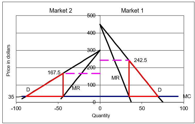
Figure 17.19: Price discrimination.

Source: MonopolyDWL.xls!TwoPriceDisc.

Figure 17.19 shows that the price discriminating monopolist will choose output where \(MR = MC\) in each market, then charge the highest price obtainable for that output in each market. The price in each market is indicated by the dashed line and it is clear that price is higher in Market 1. This makes sense because demand is more inelastic in Market 1. Those consumers are less price sensitive and the monopolist takes advantage of this to generate higher profits.

STEP To easily compare the results of the single-price monopolist in the Monopoly sheet to the price discriminator in the TwoPriceDisc sheet, click the button.

The price discriminator has the same total output, but it splits the single price into two prices. Cell B34 in the TwoPriceDisc sheet computes a weighted average of the two prices and it is higher than the single price of $192.50 charged by the conventional monopolist. This enables the two-price monopolist to make greater profits, as shown by the increase in PS from $12,403 to $13,028.

The monopolist will always be able to increase profits if it can split a market and keep the submarkets sealed off from each other, assuming the submarkets have different price elasticities. If so, a monopoly will charge the more inelastically demanded market a higher price and this is the source of the increase in profits.

Profits will continue to rise as markets are ever more finely subdivided. Amazon and other online retailers use your previous buying history, click behavior, and other information to serve up a personal price, just for you. Search for amazon+pricing+algorithm to learn more.

If you never heard about this before and think this is eye-opening or maybe even unfair, think about what colleges and universities do. They require their customers to provide detailed financial information about their ability to pay. They will, naturally, explain this as a benign effort to help the disadvantaged, but you should be glad your grocery store does not do this to you when you walk in the door.

The welfare consequences of price discrimination are not as clear. Comparing cells L38 and H34 shows that DWL has increased from $6,202 to $6,514 when the monopolist separated the markets and charged different prices. Of course, the monopolist does not care about deadweight loss; she is focused on maximizing profits. We, however, use DWL to evaluate outcomes and we would rather have the single market than the two submarkets exactly because deadweight loss is higher with price discrimination.

Unfortunately, these results do not generalize so we cannot say this will always happen. Higher DWL with price discrimination is guaranteed only for linear demand functions. In general, with nonlinear demands, we cannot state with certainty the effects on output and welfare. In other words, it is possible for output to rise and DWL to fall with a two-price discriminating monopolist. The effect on output and DWL depends on the shapes of the individual market demand curves.

For a concrete scenario of price discrimination improving welfare, consider the following from Scherer, (1970, p. 259):

It is possible, for instance, that no physician would be attracted to a small town if he were required to charge the same fee to rich patients as to poor. Since profits can be increased by discriminating, the added revenue attainable through discrimination may be sufficient to make the difference between having a service provided and not having it.

Returning to the idea of subdividing the market more finely, there is a special case of price discriminating monopoly power that is a bit mystifying, but does yield a definitive result. The perfectly price discriminating monopolist has the ability to charge different prices for different output levels down to each individual consumer. This remarkable power enables the monopolist to sell every unit of output at the highest price the market will bear.

In the Monopoly sheet, the first unit goes for $348, the 100^th for $150, and the 125^th is priced at $100. The perfectly price discriminating monopolist takes every bit of consumers’ surplus, making the greatest profit possible, but does produce the socially optimal level of output. Thus, she has no deadweight loss!

Pondering the idea of perfect price discrimination and the fact that we would judge it as a socially optimal outcome cements the idea of surplus and deadweight loss. As long as someone, anyone, even if it is a single monopolist, gets the surplus, we count it as a successful outcome. Deadweight loss is tragic precisely because no one gets it. Deadweight loss vaporizes surplus and it disappears into thin air.

Monopoly Results in Market Failure

Monopoly leads to market failure because, to maximize profits, it restricts output and, therefore, this produces a misallocation of resources. The canonical monopoly graph (see Figure 17.17) has MR splitting off of D so that \(MR=MC\) is less than the optimal output where \(P=MC\).

While most people do not like monopoly because it charges higher prices than a competitive market, this is not why economists dislike the monopoly outcome. Partial equilibrium supply and demand analysis is based on maximizing consumers’ and producer’s surplus. The logic of deadweight loss rides on the idea of waste. The monopolist does not take advantage of inframarginal sales that would lower its profit, but increase society’s total surplus. Any mechanism that generates deadweight is said to fail.

Another difference in outlook is that economists do not believe monopolists are inherently bad folks. The monopolist, like the perfectly competitive firm and consumer, is optimizing. Monopolies are in a position to improve their individual outcome and they take advantage. According to the economists, put anyone of us in the same position and we do the same thing. Do not blame the monopolist; blame the market structure for the deadweight loss.

We conclude with some advanced and heretical thinking. There is another, radically different view of monopoly that is based on the work of Joseph Schumpeter (1883 - 1950). He argued monopoly was actually a good thing because he had an evolutionary, dynamic view of capitalism. Striving for monopoly drives capitalism and monopolies are toppled by new firms in a process he named creative destruction. This oxymoron conveys Schumpeter’s vision of capitalism, with entrepreneurs engaged in an epic battle of rising firms slaying established leaders.

Schumpeter’s perspective is not that of solving society’s resource allocation problem. He considered this static optimization problem to be uninteresting because it did not apply to the real world and it had been solved already. He did not believe that price competition was the real driver of capitalism’s success. For Schumpeter, the serious open problem was how and why markets generated so much innovation and growth.

One important difference between mainstream economics and Schumpeter revolves around the government’s role. Partial equilibrium analysis says monopolies should be broken up because they generate a misallocation of resources. Schumpeterians reject the need for government to intervene, arguing that dynamic competition will erode monopoly positions through entrepreneurial innovation.

Take an Industrial Organization course, an upper-level elective taught in most economics departments around the world, to learn more about monopoly, price discrimination, and Schumpeter’s ideas.

Exercises

1. To punish a monopolist, your friend suggests applying a quantity tax on the monopoly’s commodity. Is this a good idea? Explain why or why not, using the initial values of the parameters for supply and demand in the Monopoly sheet for a concrete example.
2. Another friend suggests a quantity subsidy to eliminate the deadweight loss caused by monopoly. The idea would be to shift down MC via the subsidy until output equaled the socially optimal output. Does this make sense?
3. Consider a monopoly that sells its output in two completely separated and sealed markets. Marginal cost is constant at $35 per unit.

   Inverse demand in the two markets is given by \[P_1 = 100 - 2Q_1\] \[P_2 = 300 - 3Q_2\]

   • Solve this problem via analytical methods. Report optimal quantity and price in each market. Use Word’s Equation Editor as needed.
   • Solve this problem with the TwoPriceDisc sheet. Enter the appropriate coefficients on the sheet. Take a picture of the results and paste it in a Word doc.
   • Which market has a higher price?
   • How does the price elasticity of demand in each market affect the price?
   • Which market has greater deadweight loss? How do you know?
   • How does the price elasticity of demand affect the deadweight loss?
   • The overall market demand is given by \(P = 180 - 1.2Q\). Enter the overall market demand coefficients in the Monopoly sheet and run Solver to find the optimal solution. How does price discrimination affect welfare loss?
4. Suppose that, in the long run, average cost is decreasing throughout and marginal cost is below average cost, as shown in Figure 17.20. This is called a natural monopoly. The profit-maximizing level of output for the monopolist is where \(MR = MC\). The socially optimal result is where \(P = MC\).

   Figure 17.20: Natural monopoly.

   • What is the problem with using competitive markets to achieve the socially optimal result in this situation?
   • What government policy could be used to help the market reach the social optimum?

References

The epigraph is from page 19 of Ronald Coase, The Firm, the Market and the Law (paperback edition, 1990; originally published in 1988). Coase, a Nobel Prize winner for his work on transactions costs and property rights, criticized economics for its simplified, mathematical models that were completely stripped of real-world nuance and complexity. In “The Marginal Cost Controversy” (originally published in Economica in 1946 and reprinted in The Firm, the Market and the Law), Coase rejected the standard view that everywhere decreasing average cost (as in Figure 17.20) implied government intervention was the only solution.

Like Schumpeter, Coase has a broader, less mathematical view of economic analysis. Coase says on page 20 of The Firm, the Market and the Law,

Blackboard economics is undoubtedly an exercise requiring great intellectual ability, and it may have a role in developing the skills of an economist, but it misdirects our attention when thinking about economic policy. For this we need to consider the way in which the economic system would work with alternative institutional structures. And this requires a different approach from that used by most modern economists

Visit www.hetwebsite.net/het/profiles/schumpeter.htm for more on Schumpeter. His most accessible work is Capitalism, Socialism and Democracy.

F. M. Scherer’s Industrial Market Structure and Economic Performance came out in 1970 and was an instant classic Industrial Organization textbook. It was by far the most popular text of its day.

Today, almost all IO courses and books begin with a review of perfect competition and its polar opposite monopoly, but most of the course is about the complicated, fascinating, and vast area in between. Once you get past perfect competition and monopoly, the ways in which firms interact, compete, and strategize, is truly amazing.