19: Conclusion

1. Excel’s Solver

Consider a perfectly competitive (PC) firm with a total cost function given by \(TC=100q^{\frac{1}{2}} \). Dividing both sides by q gives us the average cost function, \(ATC=100q^{-\frac{1}{2}} \). Taking the derivative of TC with respect to q yields \(MC=50q^{-\frac{1}{2}}\).

If this PC firm faced a market price of $5/unit, what is the profit-maximizing level of output?

This book has solved optimization problems via numerical and analytical methods. We will apply both methods to this problem. First, we will use Solver.

But we will not use a prepared Excel workbook. Instead, you will create your own implementation of this problem. There are, of course, helpful steps to guide you.

STEP Open a blank Excel workbook. In cell A1, type the word quantity. Cell B1 will hold a number that represents the quantity. In cell A2, type the word profits. In cell B2, enter the formula for profit.

The price is $5/unit and \(TC=100q\) so the formula in cell B2 is: =5*B1−100*SQRT(B1).

STEP Run Solver. The target cell is B2, the goal is obviously to maximize profits, and the changing cell is B1. There are no constraints because the PC firm is free to produce as much output as it wants at the given price

Excel gives a miserable result. Depending on your Solver defaults, it might go negative and, since Excel cannot take the square root of a negative number, it gives up and announces its failure.

If so, make A1 zero and run Solver again, but this time, check the Make Unconstrained Variables Non-negative option. Your Solver may be set up so the Make Unconstrained Variables Non-negative option was already checked so you might not see the first miserable result.

Starting from zero (or a blank cell) in A1, with the non-negativity constraint, Solver says the answer is zero. This is worrisome. Could the optimal quantity really be zero?

Maybe the issue is that we are starting from blank cell, which is zero. This is poor practice. Excel interprets blanks as a zero and the formula in B1 evaluates to zero. Treating blanks as zero is one of the most dangerous things a spreadsheet does (Google sheets behaves the same way). You should always avoid this.

We can change where Solver starts from to see if that helps.

STEP Change cell B1 to 25. Cell B2 should display −375. Run Solver.

Solver appears convinced that the optimal solution is zero. We turn to analytical methods to see if we can confirm Solver’s result.

We know \(MC=50q^{-\frac{1}{2}}\) and since it is a PC firm MR = P so MR = 5. We can set MR = MC and solve for optimal q. \[5=50q^{-\frac{1}{2}} \rightarrow q^{\frac{1}{2}} = 10 \rightarrow q* = 100 \nonumber \]

This is confusing. We now have two answers: q = 0 and q = 100. Which one is correct?

Maybe a graph will help. We can draw the canonical graph of the firm’s output profit maximization problem. Figure IV.1 shows the cost curves and we can clearly see that MR = MC yields a negative profit rectangle.

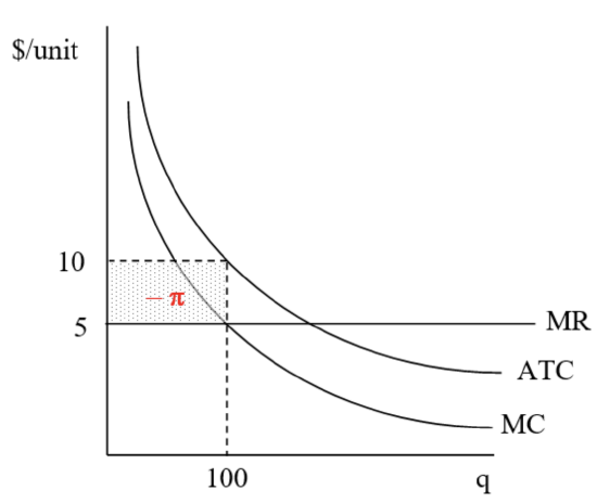
This graph helps explain what is going on here, but we need a better visual. This book claimed that looking directly at the profit function made clear the Shutdown Rule so let’s try that approach.

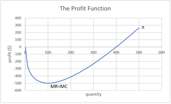
STEP Create a column from 0 to 500 by 10. This is the quantity. Use the profit formula to create a column for profit based on the quantity. Create a graph of the two columns.

If you get stuck, this 2-minute video at vimeo.com/425873093 shows how to do it.

Figure IV.2 shows the graph made in the video. It makes clear that the point where MR = MC is actually a point of minimum profit. Although the first-order condition is met (we did find a flat spot on the profit function at q = 100), this solution fails the second-order condition for a maximum.

Thus, the correct answer is to produce an infinity of output. Profits rise as more is produced past 100 units of output. Higher output leading to greater profit continues forever so the optimal solution is infinity.

How can we explain Solver’s answer of zero? Why doesn’t it give us the correct answer? When Solver starts from below 100 (we started from zero and 25), it goes to zero (or negative output if you do not have a non-negativity constraint). What happens if it starts from a number greater than 100?

STEP Enter 110 in cell A1 and run Solver.

Solver reports that “Objective cells do not converge.” Is this a miserable result? No, actually, it is the correct answer! When Solver starts from more than 100, it goes right on the \(x\) axis and profits rise and it keeps going and going. As we know, this is the right answer.

It is worth remembering that Solver’s algorithm is naive. It evaluates the function at the starting value, then moves left and right. The size of the move depends on the numerical values in the problem. Starting from q = 25, for example, Solver moves a little bit right, sees that profits fell, then goes in the opposite direction and lowers output. You can see Solver’s steps by checking the Show Iteration Results option after clicking the Options button in the Solver dialog box.

You might be thinking that since we are in the long run, ATC = AVC and it is clear that P < AVC at MR = MC, which means the firm should shut down. That is not bad thinking, except the rule does not work at MR = MC in this case because that is not the profit-maximizing output.

The takeaway of this final example is that you have to know what you are doing with Solver. It is not perfect and you cannot blindly rely on its results. This example shows that numerical methods are to be used with caution. Be careful out there.

2. Overall View

This book covered modern-day, orthodox microeconomic theory at the college undergraduate level. It used Excel to present difficult material and showed how mathematics can be used to solve problems in economics.

The economic approach or economic way of thinking provided the framework for analyzing observed behavior. The basic idea is to set up and solve an optimization problem or equilibrium model. Next, a single variable is changed, ceteris paribus, and the new solution is compared to the initial solution. This procedure is called comparative statics. Elasticity captures the logic of comparative statics in a single number.

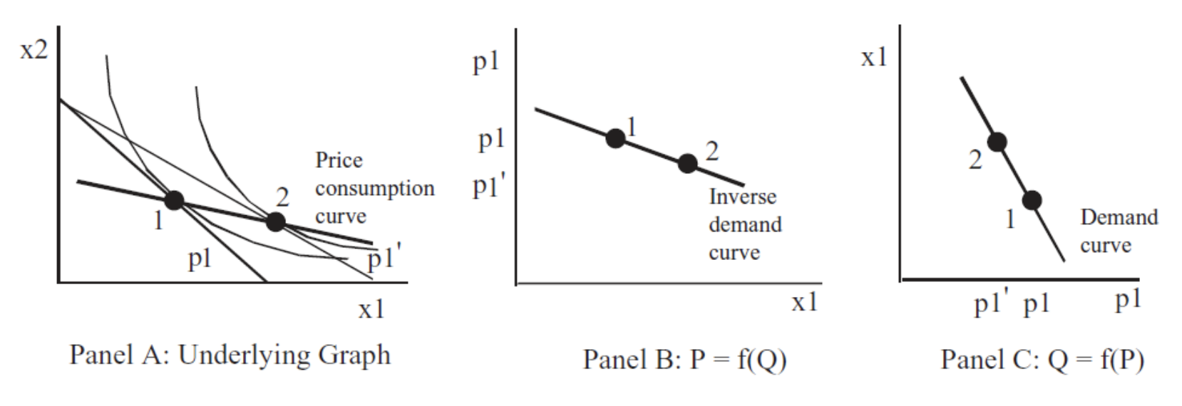
When the economic approach is applied to consumers, it is called the Theory of Consumer Behavior. The key comparative statics analysis is deriving the demand curve. Figure IV.3 is a canonical graph of deriving demand.

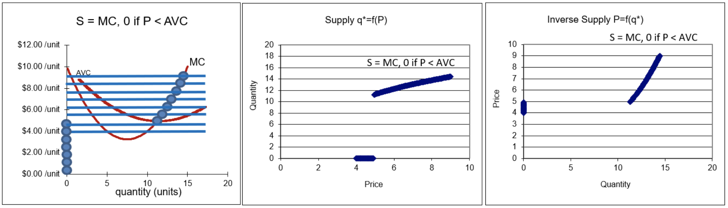
When the economic approach is applied to producers, it is called the Theory of the Firm. The key comparative statics analysis is deriving the supply curve. Figure IV.4 is a canonical graph of deriving supply.

The firm is more complicated than the consumer because firms hire inputs to produce output. In fact, the firm is really a set of three interrelated optimization problems: input cost minimization, output profit maximization, and input profit maximization.

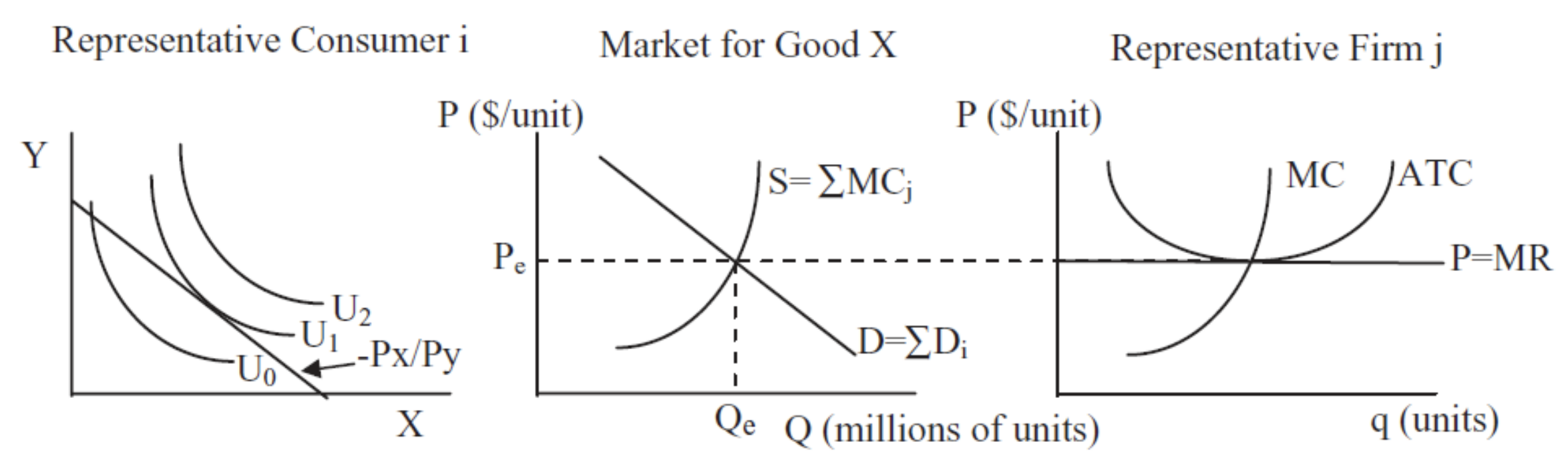
The individual demand and supply curves derived from the consumer and firm models can be added up to produce market demand and supply curves. This enables a partial equilibrium analysis of how markets solve society’s resource allocation question. Figure IV.5 shows supply and demand flanked by its consumer and firm source graphs.

Price ceilings, taxes, monopoly, import quotas, and externalities are all examples of situations where we have a misallocation of resources in a single market.

Partial equilibrium enables calculation of a measure of inefficiency called deadweight loss (also known as the Harberger triangle), but this should be interpreted as an approximation because consumers’ surplus requires that an adjustment be made to the ordinary demand curve (compensated demand must be used) and the effects on other markets are ignored. Partial equilibrium analysis is commonly used in empirical work. Think of deadweight loss as a rough measure of inefficiency in the allocation of resources.

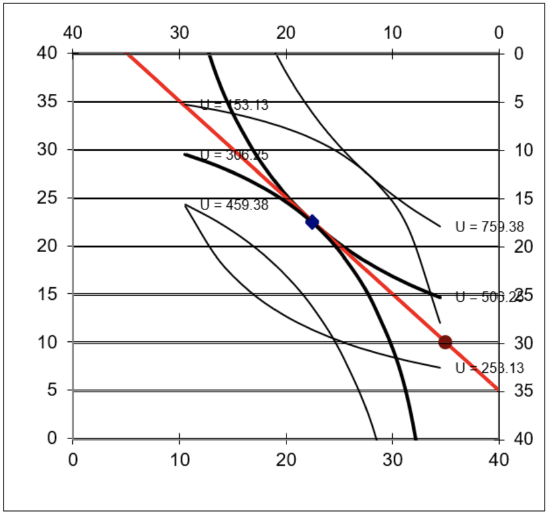
General equilibrium is a more rigorous and sophisticated analysis because it looks at all markets as a total system. Pareto’s criteria show that a properly functioning market yields an optimal allocation and monopoly is not Pareto optimal. Figure IV.6 is the canonical graph of a market’s general equilibrium and it makes clear that the market’s allocation has no Pareto Superior points.

General equilibrium does not suffer from the same problems as partial equilibrium, but it is much harder to implement in the real world. In the epigraph to the section introducing the Edgeworth Box, mention was made of computable general equilibrium models. This shows that there is an empirical side to general equilibrium analysis, but it is a relatively modern development.

It is reasonable to view mainstream microeconomics as a theory of the price mechanism. The market system uses prices as signals to allocate resources. Optimizing agents react to price changes and their interactions as buyers and sellers drive the system toward equilibrium. The Theories of Consumer Behavior and the Firm are stepping stones that explain how the market answers society’s resource allocation question. Figure IV.5 puts the Theory of Consumer Behavior, Theory of the Firm, and partial equilibrium analysis together. These three graphs and how they fit together are worth remembering.

Another organization of microeconomics splits it into two parts—individual agents (consumers and firms) that optimize and what happens when these optimizing agents interact in a market. The former is about optimization and the latter is about equilibrium. The order that is spontaneously generated by interacting, optimizing agents is a remarkable result. Economists see supply and demand not as the simple intersection of two lines, but as a pattern that is unwittingly generated by the agents themselves—just like geese that fly in a V.

This book was designed to provide you with practice in applying the economic approach. We tackled unconstrained and constrained optimization problems, computed many different elasticities, and solved several equilibrium models at the partial and general levels.

The many applications of the economic approach demonstrate its remarkable flexibility. The Theory of Consumer Behavior, at first, seems ridiculously unrealistic—a robot consumer chooses between two goods with prices, tastes, and income given! But that is just the basic model. By changing the goods to consumption in the present and the future, it becomes an intertemporal choice model. We analyzed charitable giving, portfolio theory, and the effect of safety features in automobiles with the Theory of Consumer Behavior.

In every application, the economic way of thinking was prominent. We set up and solved an optimization problem, then changed a variable, ceteris paribus, to see how the optimal solution changed. There are countless applications of the economic approach, but they share the same framework and logic.

In fact, the economic approach is what defines economics today. It may be the only discipline that defines itself by a methodology instead of by what it studies. Most people have a content-based definition of economics: They think that the study of interest rates, unemployment, and money is economics. But this is wrong. The proper definition of economics is the application of the economic approach to explain observed behavior. Crime, marriage, and war, if analyzed with the economic approach, fall under the heading of economics.

From now on, when you hear the phrase “an economic analysis of,” you will know that the economic approach is about to be applied, you will know what to expect, and you will be comfortable as the speaker talks about constraints, optimality, comparative statics, and elasticity.

3. An Open Problem

Neither this book nor modern, mainstream economics explains the dynamic process of capitalism. A few hundred years of the market system make it obvious that creativity, innovation, and technological change are endogenously generated by market-based societies. No one really knows why.

The question has been with economics since the very beginning. Many people know that Adam Smith wrote a book called the Wealth of Nations, but only a few know that the actual title is, An Inquiry into the Nature of Causes of the Wealth of Nations. But what was Smith’s inquiry, simply put?

He wanted to know why England was so much richer than its neighbors. In 1776, Smith could see British wealth all around him. He could see the economy taking off and he wondered why some places develop and grow, while others cannot seem to do so? This question remains unanswered and, in the language of mathematics, it is the biggest open problem in economics.

Explaining the dynamism of the market system is a much different question than the static optimization and equilibrium models that explain why markets allocate resources efficiently. In the static world, there are no new products, cost-saving innovations, or new firms. The static world is stable and markets are in equilibrium.

This static model clashes violently with reality. Joseph Schumpeter’s portrayal of what he called plausible (i.e., real-world) capitalism, captured in the oxymoron “creative destruction,” highlights the rise and fall of firms, explosive growth, and dislocation produced by markets. For Schumpeter, the driving force is the entrepreneur, a hero whose desire to dominate the business world results in economic success for society. But Schumpeter’s story (best captured in Capitalism, Socialism and Democracy, originally published in 1942), thrilling though it may be, is not part of mainstream economics today.

It is plainly clear that markets do generate spectacular economic growth, unparalleled by any other organizational form. Even the harshest critics of capitalism concede this point:

The bourgeoisie, during its rule of scarce one hundred years, has created more massive and more colossal productive forces than have all preceding generations together. Subjection of Nature’s forces to man, machinery, application of chemistry to industry and agriculture, steam-navigation, railways, electric telegraphs, clearing of whole continents for cultivation, canalisation of rivers, whole populations con-jured out of the ground—what earlier century had even a presentiment that such productive forces slumbered in the lap of social labour?

That was written by Karl Marx and Friedrich Engels in The Communist Manifesto in 1848, available at www.marxists.org/archive/marx/works/download /pdf/Manifesto.pdf.

Marx and Engels argued capitalism will self-destruct, but not because it failed to make goods and services. They thought it was the most productive system ever devised. They were amazed by capitalism’s ability to generate output.

Marx and Engels were not the first nor the last to be awed by the productive power of the market system. Yet, even though we can easily see that productive power, we simply do not know the answer to basic questions about how markets generate growth. Beyond superficial generalities about the institutional environment, such as needing rule of law and established property rights, we have no explanation for how the interaction of multitudes of agents drives the system over time. We cannot even answer the most basic question, posed by Adam Smith—why are some countries rich and others poor?

If we knew how and why markets caused technological change and output per person to grow exponentially, we would know how to help those societies mired in poverty. Nobel Prize winning economist Robert Lucas poses the issue this way:

Is there some action a government of India could take that would lead India’s economy to grow like Indonesia’s or Egypt’s? If so, what, exactly? If not, what is it about ‘the nature of India’ that makes it so? The consequences for human welfare involved in questions like these are simply staggering: Once one starts to think about them, it is hard to think about anything else. (Lucas, 1988, p. 5)

The point is this: Markets can be analyzed from static and dynamic perspectives. The former focuses on resource allocation at a single moment in time. It freezes the movie and asks how markets work in this motionless environment. We know how markets work as a resource allocation mechanism.

The latter perspective is about the dynamic nature of markets, we want to know how markets work over time. The movie runs—spurts of rapid growth are followed by recessions, then more growth, but output per person trends upward. Will this continue? We do not know. How do the institutions we rely on (including property rights) emerge from the interaction of optimizing agents? We do not know.

Explaining markets as a dynamic process remains the most important open problem in economics. Perhaps you can work on it.

References

The epigraph is from pages 14 and 15 of Lionel Robbins, An Essay on the Nature and Significance of Economic Science (originally published in 1932) and available online at mises.org/library/essay-nature-and-significance-economicscience.

We began with a famous quotation from Robbins, defining economics as “the science which studies human behavior as a relationship between given ends and scarce means which have alternative uses.” This book takes this definition seriously and has stressed static optimization, but this last chapter makes clear that we have a great deal to discover and learn about dynamics and technological progress.

Robert Lucas, “On the Mechanics of Economic Development,” Journal of Monetary Economics, Vol. 22 (1988), pp. 3–42, www.sciencedirect.com/sci ence/article/abs/pii/0304393288901687.

The fact that perfect competition is incompatible with increasing returns (as the Solver example with \(TC=100q^{\frac{1}{2}}\) showed) led to a heated debate in the 1920s. Economics continues to struggle to develop a model that combines the fact that average cost falls as output rises for many products with competitive markets. See David Warsh (2006), Knowledge and the Wealth of Nations: A Story of Economic Discovery, for a review of how economics has grappled with the issue of increasing returns.

If you are interested in the trajectory of capitalism and markets, then modern economic theory will not be of much help. For an entertaining review of capitalism and how it has been treated in economics, no one has beaten this classic: Robert Heilbroner, The Worldly Philosophers: The Lives, Times, and Ideas of the Great Economic Thinkers (New York: Touchstone, 1999, 7th edition, originally published 1953).