Learn how the magnification effect for quantities represents a generalization of the Rybczynski theorem by incorporating the relative magnitudes of the changes.
The magnification effect for quantities is a more general version of the Rybczynski theorem. It allows for changes in both endowments simultaneously and allows a comparison of the magnitudes of the changes in endowments and outputs.
The simplest way to derive the magnification effect is with a numerical example.
Suppose the exogenous variables of the model take the values in Table \(\PageIndex{1}\) for one country.
Table \(\PageIndex{1}\): Numerical Values for Exogenous Variables
\(a_{LC} = 2 \)
\( a_{LS} = 3 \)
\(L = 120 \)
\( a_{KC} = 1 \)
\( a_{KS} = 4 \)
\( K = 120 \)
where
\(L\) = labor endowment of the country
\(K\) = capital endowment of the country
\(a_{LC}\) = unit labor requirement in clothing production
\(a_{KC}\) = unit capital requirement in clothing production
\(a_{LS}\) = unit labor requirement in steel production
\(a_{KS}\) = unit capital requirement in steel production
With these numbers, \( \frac{a_{KS}}{a_{LS}} \left( \frac{4}{3} \right) >\frac{a_{KC}}{a_{LC}} \left( \frac{1}{2} \right) \), which means that steel production is capital intensive and clothing is labor intensive.
The following are the labor and capital constraints:
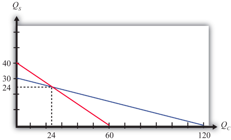
Labor constraint: \( 2Q_C + 3Q_S = 120 \)
Capital constraint: \( Q_C + 4Q_S = 120 \)
We graph these in Figure \(\PageIndex{1}\). The steeper red line is the labor constraint and the flatter blue line is the capital constraint. The output quantities on the PPF can be found by solving the two constraint equations simultaneously.
Figure \(\PageIndex{1}\): Numerical Labor and Capital Constraints
A simple method to solve these equations follows.
First, multiply the second equation by (−2) to get
\[ 2Q_C + 3Q_S = 120 \nonumber \]
and
\[ −2Q_C − 8Q_S = −240 \nonumber .\]
Adding these two equations vertically yields
\[ 0Q_C − 5Q_S = −120 \nonumber ,\]
which implies \( Q_S = \frac{-120}{-5} = 24 \). Plugging this into the first equation above (any equation will do) yields \( 2Q_C + 3 \times 24 = 120 \). Simplifying, we get \(Q_C = 120 − 722 = 24 \). Thus the solutions to the two equations are \(Q_C = 24\) and \(Q_S = 24 \).
Next, suppose the capital endowment, \(K\), increases to 150. This changes the capital constraint but leaves the labor constraint unchanged. The labor and capital constraints now are the following:
Labor constraint: \( 2Q_C + 3Q_S = 120 \)
Capital constraint: \( Q_C + 4Q_S = 150 \)
Follow the same procedure to solve for the outputs in the new full employment equilibrium.
First, multiply the second equation by (−2) to get
\[ 2Q_C + 3Q_S = 120 \nonumber \]
and
\[ −2Q_C − 8Q_S = −300 \nonumber .\]
Adding these two equations vertically yields
\[ 0Q_C − 5Q_S = −180 \nonumber ,\]
which implies \( Q_S= −180 − 5 = 36 \). Plugging this into the first equation above (any equation will do) yields \(2Q_C + 3 \times 36 = 120\). Simplifying, we get \(Q_C = \frac{120 − 108}{2} = 6\). Thus the new solutions are \(Q_C = 6\) and \(Q_S = 36\).
The Rybczynski theorem says that if the capital endowment rises, it will cause an increase in output of the capital-intensive good (in this case, steel) and a decrease in output of the labor-intensive good (clothing). In this numerical example, \(Q_S\) rises from 24 to 36 and \(Q_C\) falls from 24 to 6.
Percentage Changes in the Endowments and Outputs
The magnification effect for quantities ranks the percentage changes in endowments and the percentage changes in outputs. We’ll denote the percentage change by using a ^ above the variable (i.e., \( \hat X \) = percentage change in \(X\)).
Table \(\PageIndex{2}\): Calculating Percentage Changes in the Endowments and Outputs
\( \hat K = \frac{150−120}{120} \times 100 = +25\% \)
The rank order of the changes in Table \(\PageIndex{2}\) is the magnification effect for quantities:
\[ \hat Q_S > \hat K > \hat L > \hat Q_C \nonumber .\]
The effect is initiated by changes in the endowments. If the endowments change by some percentage, ordered as above, then the quantity of the capital-intensive good (steel) will rise by a larger percentage than the capital stock change. The size of the effect is magnified relative to the cause.
The quantity of cloth (\(Q_C\)) changes by a smaller percentage than the smaller labor endowment change. Its effect is magnified downward.
Although this effect was derived only for the specific numerical values assumed in the example, it is possible to show, using more advanced methods, that the effect will arise for any endowment changes that are made. Thus if the labor endowment were to rise with no change in the capital endowment, the magnification effect would be
\[ \hat Q_C > \hat L > \hat K > \hat Q_S \nonumber .\]
This implies that the quantity of the labor-intensive good (clothing) would rise by a greater percentage than the quantity of labor, while the quantity of steel would fall.
The magnification effect for quantities is a generalization of the Rybczynski theorem. The effect allows for changes in both endowments simultaneously and provides information about the magnitude of the effects. The Rybczynski theorem is one special case of the magnification effect that assumes one of the endowments is held fixed.
Although the magnification effect is shown here under the special assumption of fixed factor proportions and for a particular set of parameter values, the result is much more general. It is possible, using calculus, to show that the effect is valid under any set of parameter values and in a more general variable proportions model.
Key Takeaways
The magnification effect for quantities shows that if the factor endowments change by particular percentages with one greater than the other, then the outputs will change by percentages that are larger than the larger endowment change and smaller than the smaller. It is in this sense that the output changes are magnified relative to the factor changes.
If the percentage change of the capital endowment exceeds the percentage change of the labor endowment, for example, then output of the good that uses capital intensively will change by a greater percentage than capital changed, while the output of the good that uses labor intensively will change by less than labor changed.
Exercise \(\PageIndex{1}\)
Consider a two-factor (capital and labor), two-good (beer and peanuts) H-O economy. Suppose beer is capital intensive. Let \(Q_B\) and \(Q_P\) represent the outputs of beer and peanuts, respectively.
Write the magnification effect for quantities if the labor endowment increases and the capital endowment decreases
Write the magnification effect for quantities if the capital endowment increases by 10 percent and the labor endowment increases by 5 percent.
Write the magnification effect for quantities if the labor endowment decreases by 10 percent and the capital endowment decreases by 15 percent.
Write the magnification effect for quantities if the capital endowment decreases while the labor endowment does not change.
Consider a country producing milk and cookies using labor and capital as inputs and described by a Heckscher-Ohlin model. The following table provides outputs for goods and factor endowments before and after a change in the endowments.
Table \(\PageIndex{3}\): Outputs and Endowments
Initial
After Endowment Change
Milk Output (\(QM\))
100 gallons
110 gallons
Cookie Output (\(QC\))
100 pounds
80 pounds
Labor Endowment (\(L\))
4,000 hours
4,200 hours
Capital Endowment (\(K\))
1,000 hours
1,000 hours
Calculate and display the magnification effect for quantities in response to the endowment change.
Which product is capital intensive?
Which product is labor intensive?
Consider the following data in a Heckscher-Ohlin model with two goods (wine and cheese) and two factors (capital and labor).
\(a_{KC}\) = 5 hours per pound (unit capital requirement in cheese)
\(a_{KW}\) = 10 hours per gallon (unit capital requirement in wine)
\(a_{LC}\) = 15 hours per pound (unit labor requirement in cheese)
\(a_{LW}\) = 20 hours per gallon (unit labor requirement in wine)
\(L\) = 5,500 hours (labor endowment)
\(K\) = 2,500 hours (capital endowment)
Solve for the equilibrium output levels of wine and cheese.
Suppose the labor endowment falls by 100 hours to 5,400 hours. Solve for the new equilibrium output levels of wine and cheese.
Calculate the percentage changes in the outputs and endowments and write the magnification effect for quantities.
Identify which good is labor intensive and which is capital intensive.