3.1: Elasticity

Learning Objectives

• What is the best way of measuring the responsiveness of demand?
• What is the best way of measuring the responsiveness of supply?

Let \(x (p)\) represent the quantity purchased when the price is p, so that the function x represents demand. How responsive is demand to price changes? One might be tempted to use the derivative, \(x′\), to measure the responsiveness of demand, since it measures how much the quantity demanded changes in response to a small change in price. However, this measure has two problems. First, it is sensitive to a change in units. If I measure the quantity of candy in kilograms rather than in pounds, the derivative of demand for candy with respect to price changes even if the demand itself is unchanged. Second, if I change price units, converting from one currency to another, again the derivative of demand will change. So the derivative is unsatisfactory as a measure of responsiveness because it depends on units of measure. A common way of establishing a unit-free measure is to use percentages, and that suggests considering the responsiveness of demand to a small percentage change in price in percentage terms. This is the notion of elasticity of demand. The concept of elasticity was invented by Alfred Marshall (1842–1924) in 1881 while sitting on his roof. The elasticity of demand is the percentage decrease in quantity that results from a small percentage increase in price. Formally, the elasticity of demand, which is generally denoted with the Greek letter epsilon, ε, (chosen mnemonically to indicate elasticity) is

\begin{equation}\varepsilon=-d x x d p p=-p x d x d p=-p x^{\prime}(p) x(p)\end{equation}

The minus sign is included in the expression to make the elasticity a positive number, since demand is decreasing. First, let’s verify that the elasticity is, in fact, unit free. A change in the measurement of x doesn’t affect elasticity because the proportionality factor appears in both the numerator and denominator. Similarly, a change in the measure of price so that p is replaced by r = ap, does not change the elasticity, since as demonstrated below,

\begin{equation}\varepsilon=-r d d r x(r / a) x(r / a)=-r x^{\prime}(r / a) 1 a x(r / a)=-p x^{\prime}(p) x(p)\end{equation}

the measure of elasticity is independent of a, and therefore not affected by the change in units.

How does a consumer’s expenditure, also known as (individual) total revenue, react to a change in price? The consumer buys x(p) at a price of p, and thus total expenditure, or total revenue, is TR = px(p). Thus,

\begin{equation}d \text { dp } p x(p)=x(p)+p x^{\prime}(p)=x(p)\left(1+p x^{\prime}(p) x(p)\right)=x(p)(1-\varepsilon)\end{equation}

Therefore,

\[d dp TR 1 p TR =1−ε. \nonumber \]

In other words, the percentage change of total revenue resulting from a 1% change in price is one minus the elasticity of demand. Thus, a 1% increase in price will increase total revenue when the elasticity of demand is less than one, which is defined as an inelastic demand. A price increase will decrease total revenue when the elasticity of demand is greater than one, which is defined as an elastic demand. The case of elasticity equal to one is called unitary elasticity, and total revenue is unchanged by a small price change. Moreover, that percentage increase in price will increase revenue by approximately 1 – ε percent. Because it is often possible to estimate the elasticity of demand, the formulae can be readily used in practice. Table 3.1 provides estimates on demand elasticities for a variety of products.

Table 3.1 Various Demand Elasticities

Product	Product	ε
Salt	Movies	0.9
Matches	Shellfish, consumed at home	0.9
Toothpicks	Tires, short-run	0.9
Airline travel, short-run	Oysters, consumed at home	1.1
Residential natural gas, short-run	Private education	1.1
Gasoline, short-run	Housing, owner occupied, long-run	1.2
Automobiles, long-run	Tires, long-run	1.2
Coffee	Radio and television receivers	1.2
Legal services, short-run	Automobiles, short-run	1.2-1.5
Tobacco products, short-run	Restaurant meals	2.3
Residential natural gas, long-run	Airline travel, long-run	2.4
Fish (cod) consumed at home	Fresh green peas	2.8
Physician services	Foreign travel, long-run	4.0
Taxi, short-run	Chevrolet automobiles	4.0
Gasoline, long-run	Fresh tomatoes	4.6

From http://www.mackinac.org/archives/1997/s1997-04.pdf; cited sources: James D. Gwartney and Richard L. Stroup,, Economics: Private and Public Choice, 7th ed., 1995; 8th ed., 1997; Hendrick S. Houthakker and Lester D. Taylor, Consumer Demand in the United States, 1929–1970 (1966; Cambridge: Harvard University Press, 1970); Douglas R. Bohi, Analyzing Demand Behavior (Baltimore: Johns Hopkins University Press, 1981); Hsaing-tai Cheng and Oral Capps, Jr., "Demand for Fish," American Journal of Agricultural Economics, August 1988; and U.S. Department of Agriculture.

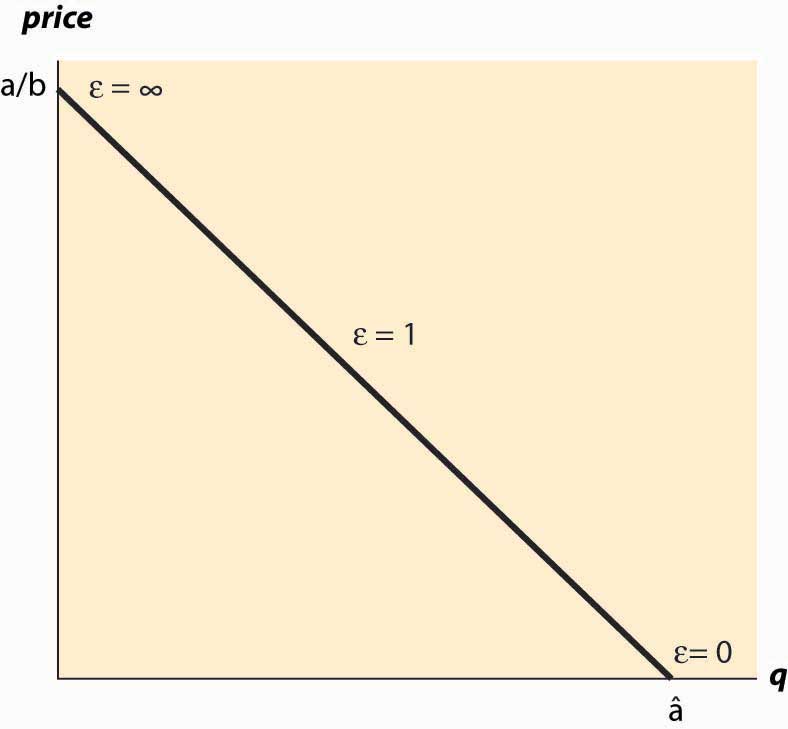
When demand is linear, \(\begin{equation}x(p)=a-b p\end{equation}\), the elasticity of demand has the form

\begin{equation}\varepsilon=\mathrm{bp} \mathrm{a}-\mathrm{bp}=\mathrm{p} \text { a } \mathrm{b}-\mathrm{p}\end{equation}

This case is illustrated in Figure 3.1.

Figure 3.1 Elasticities for linear demand

If demand takes the form x(p) = a * p^−ε, then demand has constant elasticity, and the elasticity is equal to ε. In other words, the elasticity remains at the same level while the underlying variables (such as price and quantity) change.

The elasticity of supply is analogous to the elasticity of demand in that it is a unit-free measure of the responsiveness of supply to a price change, and is defined as the percentage increase in quantity supplied resulting from a small percentage increase in price. Formally, if s(p) gives the quantity supplied for each price p, the elasticity of supply, denoted by η (the Greek letter “eta,” chosen because epsilon was already taken) is

\begin{equation}\eta=\operatorname{ds} \mathrm{s} \mathrm{dp} \mathrm{p}=\mathrm{p} \mathrm{s} \mathrm{ds} \mathrm{dp}=\mathrm{ps}^{\prime}(\mathrm{p}) \mathrm{s}(\mathrm{p})\end{equation}

Again, similar to demand, if supply takes the form s(p) = a * p^η, then supply has constant elasticity, and the elasticity is equal to η. A special case of this form is linear supply, which occurs when the elasticity equals one.

Key Takeaways

• The elasticity of demand is the percentage decrease in quantity that results from a small percentage increase in price, which is generally denoted with the Greek letter epsilon, ε.
• The percentage change of total revenue resulting from a 1% change in price is one minus the elasticity of demand.
• An elasticity of demand that is less than one is defined as an inelastic demand. In this case, increasing price increases total revenue.
• A price increase will decrease total revenue when the elasticity of demand is greater than one, which is defined as an elastic demand.
• The case of elasticity equal to one is called unitary elasticity, and total revenue is unchanged by a small price change.
• If demand takes the form x (p) = a * p^−ε , then demand has constant elasticity, and the elasticity is equal to ε.
• The elasticity of supply is defined as the percentage increase in quantity supplied resulting from a small percentage increase in price.
• If supply takes the form s (p) = a * p ^η, then supply has constant elasticity, and the elasticity is equal to η.

EXERCISES

1. Suppose a consumer has a constant elasticity of demand ε, and demand is elastic \(\begin{equation}(ε > 1)\end{equation}\). Show that expenditure increases as price decreases.
2. Suppose a consumer has a constant elasticity of demand ε, and demand is inelastic \(\begin{equation}(ε < 1)\end{equation}\). What price makes expenditure the greatest?
3. For a consumer with constant elasticity of demand \(\begin{equation}(ε > 1)\end{equation}\), compute the consumer surplus.
4. For a producer with constant elasticity of supply, compute the producer profits.