7.7: Aggregate demand and equilibrium output

Last updated
Save as PDF

Page ID: 45776

\( \newcommand{\vecs}[1]{\overset { \scriptstyle \rightharpoonup} {\mathbf{#1}} } \) \( \newcommand{\vecd}[1]{\overset{-\!-\!\rightharpoonup}{\vphantom{a}\smash {#1}}} \)\(\newcommand{\id}{\mathrm{id}}\) \( \newcommand{\Span}{\mathrm{span}}\) \( \newcommand{\kernel}{\mathrm{null}\,}\) \( \newcommand{\range}{\mathrm{range}\,}\) \( \newcommand{\RealPart}{\mathrm{Re}}\) \( \newcommand{\ImaginaryPart}{\mathrm{Im}}\) \( \newcommand{\Argument}{\mathrm{Arg}}\) \( \newcommand{\norm}[1]{\| #1 \|}\) \( \newcommand{\inner}[2]{\langle #1, #2 \rangle}\) \( \newcommand{\Span}{\mathrm{span}}\) \(\newcommand{\id}{\mathrm{id}}\) \( \newcommand{\Span}{\mathrm{span}}\) \( \newcommand{\kernel}{\mathrm{null}\,}\) \( \newcommand{\range}{\mathrm{range}\,}\) \( \newcommand{\RealPart}{\mathrm{Re}}\) \( \newcommand{\ImaginaryPart}{\mathrm{Im}}\) \( \newcommand{\Argument}{\mathrm{Arg}}\) \( \newcommand{\norm}[1]{\| #1 \|}\) \( \newcommand{\inner}[2]{\langle #1, #2 \rangle}\) \( \newcommand{\Span}{\mathrm{span}}\)\(\newcommand{\AA}{\unicode[.8,0]{x212B}}\)

Our objective in this chapter was to extend the model of Chapter 6 to include a government sector and fiscal policy in aggregate demand. To do this we continued to assume that wages, prices, money supply, interest rates, and foreign exchange rates are constant. We also continued to make the important distinction between autonomous expenditure and induced expenditure, which leads to the existence of a multiplier. The equilibrium condition is still Y=AE and AD=AS, output and income equal to planned expenditure. Even though the model is more complex, it still shows us that fluctuations in autonomous expenditures, working through the multiplier, cause fluctuations in Aggregate Demand, output, income, and employment.

Changes in autonomous expenditures are still the sources of business cycles. If business changes planned investment expenditure in response to changed expectations about future markets, or if changes in economic conditions in other countries change exports or imports, the multiplier translates these changes into larger changes or fluctuations in income and employment. Government expenditure plans and net tax rates are fiscal policy tools that could be used to moderate or offset these fluctuations through a combination of automatic and discretionary fiscal policy.

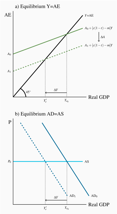
Figure 7.11 shows the relationship between equilibrium income and output, and the link between changes in aggregate expenditure, aggregate demand, and equilibrium income. In the upper diagram a fall in autonomous expenditure from A₀ to A₁ reduces AE and equilibrium Y from to , which is the fall in A times the multiplier.

The fall in autonomous expenditure and equilibrium is a leftward shift in the AD curve in the lower diagram. The size of that shift in AD is the change in equilibrium income in the upper diagram, namely the fall in A times the multiplier. Because the price level is constant, giving a horizontal AS curve at P₀, the fall in equilibrium determined by AD/AS is the same as the horizontal shift in AD.

Figure 7.11 AE, AD and equilibrium output

Example Box 7.1 The effect of the government sector on equilibrium income

a) Equilibrium with no Government
Autonomous expenditure	=A₀	Autonomous expenditure	=80
Induced expenditure	=(c–m)Y	Induced expenditure	=(0.8–0.2)Y=0.6Y
Aggregate expenditure	=A₀+(c–m)Y	Aggregate expenditure	=80+0.6Y
Equilibrium income:		Equilibrium income:
	Y=A₀+(c–m)Y		Y=80+0.6Y


			Y=200

b) Equilibrium with added government sector: G=25, NT=0.10Y
Autonomous expenditure	=A₀+G₀	Autonomous expenditure	=105
Induced expenditure	=c(1–t)–m	Induced expenditure
Aggregate expenditure		Aggregate expenditure	=105+0.52Y
Equilibrium income:		Equilibrium income:
			Y=105+0.52Y
			Y(1–0.52)=105

			Y=218.4

In this example adding government expenditure G=25 financed in part by a net tax rate t=0.10 raised autonomous expenditure by 25 but lowered the multiplier from 2.5 to 2.08 with the result that equilibrium income increased by 18.4. Equilibrium income increased because the government sector ran a budget deficit. G was 25 but net tax revenue was only .