18: Solutions
- Page ID
- 45500

\( \newcommand{\vecs}[1]{\overset { \scriptstyle \rightharpoonup} {\mathbf{#1}} } \) \( \newcommand{\vecd}[1]{\overset{-\!-\!\rightharpoonup}{\vphantom{a}\smash {#1}}} \)\(\newcommand{\id}{\mathrm{id}}\) \( \newcommand{\Span}{\mathrm{span}}\) \( \newcommand{\kernel}{\mathrm{null}\,}\) \( \newcommand{\range}{\mathrm{range}\,}\) \( \newcommand{\RealPart}{\mathrm{Re}}\) \( \newcommand{\ImaginaryPart}{\mathrm{Im}}\) \( \newcommand{\Argument}{\mathrm{Arg}}\) \( \newcommand{\norm}[1]{\| #1 \|}\) \( \newcommand{\inner}[2]{\langle #1, #2 \rangle}\) \( \newcommand{\Span}{\mathrm{span}}\) \(\newcommand{\id}{\mathrm{id}}\) \( \newcommand{\Span}{\mathrm{span}}\) \( \newcommand{\kernel}{\mathrm{null}\,}\) \( \newcommand{\range}{\mathrm{range}\,}\) \( \newcommand{\RealPart}{\mathrm{Re}}\) \( \newcommand{\ImaginaryPart}{\mathrm{Im}}\) \( \newcommand{\Argument}{\mathrm{Arg}}\) \( \newcommand{\norm}[1]{\| #1 \|}\) \( \newcommand{\inner}[2]{\langle #1, #2 \rangle}\) \( \newcommand{\Span}{\mathrm{span}}\)\(\newcommand{\AA}{\unicode[.8,0]{x212B}}\)
Solutions
Chapter 1 Solutions
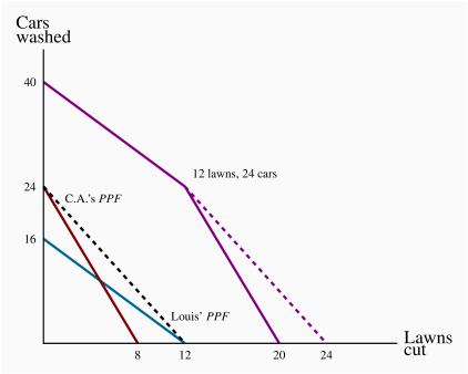
EXERCISE 1.1
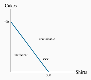
If all 100 workers make cakes their output is
 .
.If all workers make shirts their output is
 .
.
EXERCISE 1.2
EXERCISE 1.3
EXERCISE 1.4
EXERCISE 1.5
EXERCISE 1.6
EXERCISE 1.7
Chapter 2 Solutions
EXERCISE 2.1
EXERCISE 2.2
| Year | 2005 | 2006 | 2007 | 2008 | 2009 | 2010 | 2011 | 2012 | 2013 | 2014 |
| Index | 100.0 | 105.0 | 109.0 | 115.0 | 120.0 | 120.0 | 127.0 | 130.0 | 139.0 | 142.0 |
EXERCISE 2.3
EXERCISE 2.4
| Pct Inc | 1.3 | 2.7 | 2.0 | 4.0 | 2.7 | 2.0 | 3.1 |
| Pct Con | 3.0 | 1.6 | 3.7 | 3.8 | 4.1 | 4.1 | 3.4 |
EXERCISE 2.5
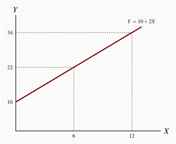
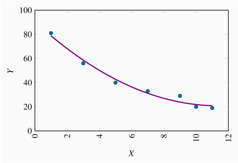
| X | 0 | 1 | 2 | 3 | 4 | 5 | 6 | 7 | 8 | 9 | 10 | 11 | 12 |
| Y | 10 | 12 | 14 | 16 | 18 | 20 | 22 | 24 | 26 | 28 | 30 | 32 | 34 |
EXERCISE 2.6
Chapter 3 Solutions
EXERCISE 3.1
EXERCISE 3.2
EXERCISE 3.3
EXERCISE 3.4
EXERCISE 3.5
EXERCISE 3.6
EXERCISE 3.7
EXERCISE 3.8
EXERCISE 3.9
EXERCISE 3.10
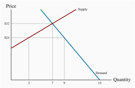
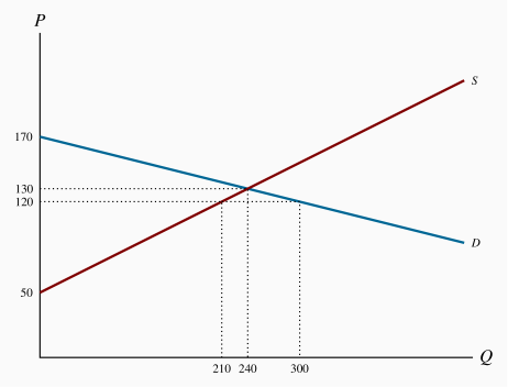
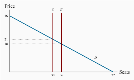
The equilibrium admission price is
 ,
,  .
.The equilibrium price would now become $18 and
 . Yes.
EXERCISE 3.11
Chapter 4 Solutions
EXERCISE 4.1