1.5: The Motivation for and Consequences of Free Trade

Introduction to Welfare Economics

Welfare economics is concerned with how well off individuals and groups are. Welfare economics is not about government programs to assist the needy… that is a different type of welfare. In economics, welfare economics is used to see how the welfare, or well-being of individuals and groups changes with a change in policies, programs, or current events.

Welfare Economics = The study and calculation of gains and losses to market participants from changes in market conditions and economic policies.

Consumer Surplus and Producer Surplus

The two most important groups that are studied in welfare economics are producers and consumers. The concepts of Consumer Surplus \((CS)\) and Producer Surplus \((PS)\) are used to measure the wellbeing of consumers and producers, respectively.

Consumer Surplus \((CS)\) = A measure of how well off consumers are. Willingness to pay minus the price actually paid.

Producer Surplus \((PS)\) = A measure of how well off producers are. Price received minus the cost of production.

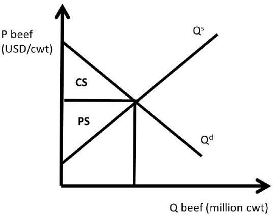
The intuition of consumer surplus provides a good method of learning the concept. Suppose that I am on my way to the store to purchase a hammer, and I think to myself, “I am willing to pay six dollars for the hammer.” When I arrive at the store, I find that the price of the hammer is four dollars. My consumer surplus is equal to two dollars: the willingness to pay minus the actual price paid. In this manner, we can add up all consumers in the market to measure consumer surplus for all consumers. This can be seen in Figure \(\PageIndex{1}\). If each point on the demand curve is considered an individual consumer, then \(CS\) is the difference between each point on the demand curve and the price line. The demand curve represents the consumers’ willingness and ability to pay for a good. The \(CS\) area is a triangle, and equal to the level of consumer surplus in the market (Figure \(\PageIndex{1}\)).

Similarly, the intuition of producer surplus is a good place to start. If a wheat producer can produce a bushel of wheat for four dollars, and she receives six dollars per bushel when she sells her wheat, then her level of producer surplus is equal to two dollars. Producer surplus is the price received minus the cost of production. In Figure \(\PageIndex{1}\), this is the difference between the price line and the supply curve. The market supply curve was derived by summing all individual firms’ marginal cost curves. Therefore, the supply curve represents the cost of production. The \(PS\) area is the area identified in Figure \(\PageIndex{1}\).

Figure \(\PageIndex{1}\): Welfare Economics of the Beef Market

These areas can be quantified, or measured, to find the dollar value of consumer surplus and producer surplus. These measures place a dollar value on the wellbeing of producers and consumers.

Mathematics of Consumer and Producer Surplus: Phone Market

Remember that the inverse supply and demand for phones was given by:

\[P = 100 – 2Q^d, \label{1.28}\]

and

\[P = 20 + 2Q^s. \label{1.29}\]

Where P is the price of phones in dollars/unit, and Q is the quantity of phones in millions. The equilibrium price and quantity of phones were calculated above in section 1.4.10:

\[\begin{align*}P^e &= \text{ USD } 60\text{/phone}\\Q^e &= 20 \text{ million phones.}\end{align*}\]

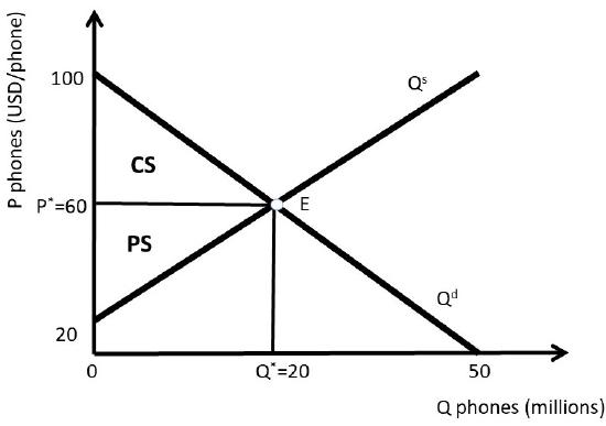
These values, together with the supply and demand functions, allow us to measure the well-being of both consumers and producers. From geometry, the area of a triangle is one half base times height. To calculate \(CS\) and \(PS\), multiply the base of the triangle times the height of the triangle in Figure \(\PageIndex{2}\), then multiply by one half, or 0.5 (Equations \ref{1.30} and \ref{1.31}).

\[\begin{align} CS &= 0.5(100 – 60)(20) = 0.5(40)(20) = 400 \text{ million USD}\label{1.30}\\PS &= 0.5(60 – 20)(20) = 0.5(40)(20) = 400 \text{ million USD}\label{1.31}\end{align}\]

We will use the concepts of consumer surplus and producer surplus extensively in what follows, where we will explore the consequences of policies, international trade, and immigration in food and agriculture.

Figure \(\PageIndex{2}\): Consumer and Producer Surplus Calculations in the Phone Market

The units for both \(CS\) and \(PS\) are in terms of dollars (USD). These measures capture how well off consumers and producers are in dollars, or the dollar value of their happiness, or well-being. The units are price units multiplied by quantity units, or \((\text{USD/phone})\cdot(\text{million phones})\). Notice that the phone units are in both the numerator and denominator, so they are cancelled, leaving million dollars.

1.6 The Motivation for and Consequences of Free Trade

The Motivation for Free Trade and Globalization

Globalization and free trade result in enormous economic benefits to nations that trade. These benefits have led to high incomes in many nations throughout the world, particularly since 1950. As with all national policies, there are benefits and costs to international trade: there are winners and losers to globalization. When trade is voluntary, the gains are mutually beneficial, and the overall benefits are greater than the costs. There is a strong motivation to trade, and the nations of the world continue to become more globalized over time.

A nation’s consumption possibilities are vastly increased with trade. In nations North of the equator such as the USA, Japan, EU, and China, fresh fruit and vegetables can be purchased during the winter from nations in the Southern hemisphere. In the United States, tropical products including coffee, sugar, bananas, cocoa, and pineapple are imported, since the costs of producing these goods are much lower in tropical climates than in the USA.

The principle of comparative advantage provides large benefits to individuals, nations, and firms that specialize in what they do best, and trade for other goods. This process greatly expands the consumption possibilities of all nations, due to efficiency gains that arise from specialization and gains from trade. For example, if Canada specializes in wheat production, and Costa Rica produces bananas, both nations could be better off through specialization and trade.

A nation that does not trade with other nations is called a closed economy.

Closed Economy = A nation that does not trade. All goods and services consumed must be produced within the nation. There are no imports or exports.

Open Economy = A nation that allows trade. Imports and exports exist.

If a nation does not trade, then consumers in the closed economy must only consume what it produces. In this case, quantity supplied must equal quantity demanded \((Q^s = Q^d)\). Trade allows this equality to be broken, providing the opportunity for imports \((Q^s < Q^d)\) or exports \((Q^s > Q^d)\). The concepts of Excess Supply and Excess Demand will be introduced in the next section to aid in understanding the motivation and consequences of free trade.

1.6.2 Excess Supply and Excess Demand

We will use wheat as an example to see how and why trade occurs. We will investigate wheat trade between the USA and Japan. Japan is one of the largest international buyers of wheat from the United States. The USA is a wheat exporter. The left panel of Figure \(\PageIndex{3}\) show the USA wheat market. Define \(P_e\) to be the price of wheat in the exporting nation. At price \(P_e\), domestic consumption \((Q_d)\) is equal to domestic production \((Q_s)\).

Figure \(\PageIndex{3}\): The Excess Supply of Wheat

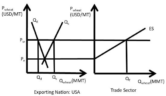
Excess supply is defined to be the quantity of exportable surplus, or \(Q^s – Q^d\). At prices higher than \(P_e\), the quantity supplied becomes greater than the quantity demanded, and excess supply exists.

Excess Supply \((ES)\) = Quantity supplied minus quantity demanded at a given price, \(Q^s – Q^d\).

At prices higher than \(P_e\), wheat producers increase the quantity supplied along the supply curve \(Q^s\) due to the Law of Supply. Wheat consumers decrease purchases of wheat along the demand curve \(Q^d\), due to the Law of Demand. The result is a surplus, or excess supply, at the higher price. If excess supply existed in a closed economy, market forces would come into play to bring the higher price back down to the market equilibrium level, \(P_e\). In an open economy, however, it is possible to maintain the high market price through exports. In the right-hand panel of Figure \(\PageIndex{3}\), the \(ES\) function represents excess supply, equal to the horizontal distance between \(Q^s\) and \(Q^d\) in the left-hand panel. Note that \(ES = 0\) at \(P_e\), and becomes larger as the price of wheat increases.

Free trade allows the USA to use its resource to produce more wheat than it consumes, and export what is left over to enhance what producer revenues. Trade also provides the opportunity to buy imported goods from other nations.

Figure \(\PageIndex{3}\): The Excess Demand of Wheat

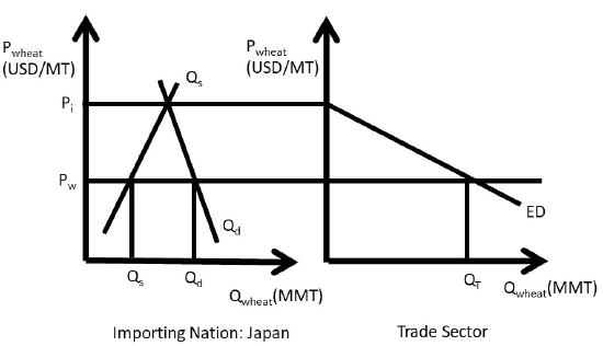
Define \(P_i\) to be the price of wheat in the importing nation (Japan in this case). An importing nation such as Japan is characterized by a price lower than the domestic market equilibrium price \((P_i)\), where \(Q^s = Q^d\) (Figure \(\PageIndex{3}\)). In an importing nation, quantity demanded is greater than quantity supplied \((Q^s < Q^d)\), and the price is lower than the market equilibrium price. If the price is lower than \(P_i\) in Figure \(\PageIndex{3}\), consumers increase purchases of the good due to the Law of Demand, and producers decrease production of the good, following the Law of Supply. This results in an Excess Demand for the good.

Excess Demand \((ED)\) = Quantity demanded minus quantity supplied at a given price, \(Q^d – Q^s\).

Note that any shift in either supply or demand of wheat in the importing nation will shift the \(ED\) curve. Domestic events in the markets for traded goods have international consequences. What happens in China has a large impact on USA wheat producers. Next, the exporting and importing nations will be linked through international trade.

The \(ED\) curve shown in the right-hand panel of Figure \(\PageIndex{3}\) represents excess demand, equal to the horizontal distance between \(Q^d\) and \(Q^s\) in the left-hand panel. Note that \(ED = 0\) at \(P_i\), and becomes larger as the price of wheat decreases.

1.6.3 Three Panel Diagram of Trade between Two Nations

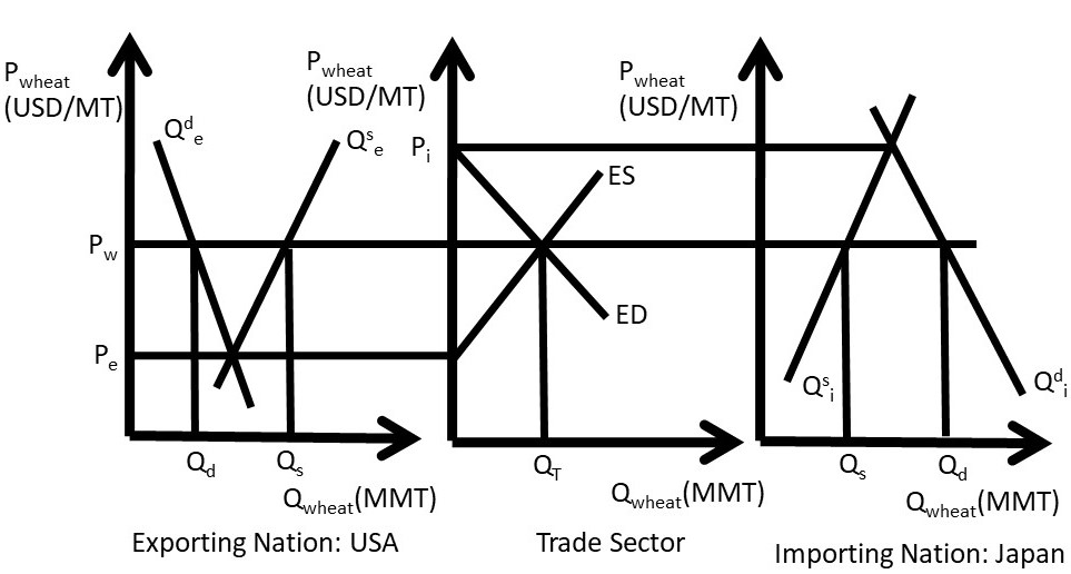
Now consider the wheat exporting nation (USA) and wheat importing nation (Japan) in the same diagram, Figure \(\PageIndex{4}\). The wheat market in the exporting nation is shown in the left panel, and the wheat market in the importing nation is shown in the right panel (Figure \(\PageIndex{4}\)). The trade sector is in the middle panel. Excess demand \((ED)\) is downward sloping, and is derived from the domestic supply \((Q^s_i)\) and demand \((Q^d_i)\) in the importing nation, Japan in this case. Excess Supply \((ES)\) is upward sloping, derived from the supply \((Q^s_e)\) and demand \((Q^d_e)\) curves in the exporting nation, the USA. In reality, the right panel is composed of many nations: all countries that import wheat. For simplicity, the model here is for one importing nation and one exporting nation. As price \((P_i)\) decreases in Japan, quantity demanded \((Q^d_i)\) increases and quantity supplied \((Q^s_i)\) decreases, causing \(ED\) to have a negative slope. Similarly, price \((P_e)\) increases in the exporting nation (USA) result in a higher quantity supplied of wheat \((Q^s_e)\) and a lower quantity demanded \((Q^d_e)\). Equilibrium in the global wheat market is found in the center panel at the point where \(ED = ES\).

The quantity of wheat traded \((Q_T)\) is equal to \(ED\) at the world price \((P_w)\), which is also equal to \(ES\) at the world price. Note that it must be true that \(ED=ES\): any imported goods in one nation must be exported by the other nation. Therefore, \(Q_T = ED = ES = (Q^d_i – Q^s_i) = (Q^s_e – Q^d_e)\).

In a multi-nation model, this equilibrium would occur when the sum of all wheat supplied from all exporting nations \((= ΣES = Q^s_e – Q^d_e)\) is equal to the sum of all wheat demanded from all importing nations \((= ΣED = Q^d_i -Q^s_i)\). The equilibrium quantity traded \((Q_T)\) is equal to the quantity of wheat imported by Japan \((ED_i)\) and the quantity of wheat exported by the USA \((ES_e)\) since exports must equal imports (\(Q_T\) = exports = imports). This equilibrium in the world market determines the world price \((P_w)\), which is the price of wheat for all trading partners, Japan and the USA in this model.

Figure \(\PageIndex{4}\): International Trade in Wheat: USA and Japan

The three-panel diagram demonstrates two important characteristics about free trade. First, the motivation for trade is simple: “buy low and sell high.” If a price difference exists between two locations, arbitrage provides profit opportunities for traders. A firm (or nation) that buys wheat at a lower price in the USA and sells the wheat at a higher price in Japan can earn profits. Note that this simple model ignores transportation costs and exchange rates. Second, anything that affects the supply or demand of wheat in either trading nation affects the global price and quantity of wheat. Therefore, all consumers and producers of a good are interconnected: the welfare of all wheat producers and consumers is affected by weather, growing conditions, food trends, and all other supply and demand determinants in all trading nations.

This point is enormously important in a globalized economy: the well-being of all producers and consumers depends on people, politicians, and current events all over the globe. The three-panel diagram is useful in understanding the determinants of food and agricultural exports: all supply and demand shifters in all wheat exporting and importing nations.