The previous chapter emphasized the market demand schedule. The demand schedule shows the relationship between the amount of a product or service demanded and its own-price. The supply schedule is analogous in that it shows the relationship between the amount of a product supplied to the market and the product’s own-price. Again, the convention will be to plot the supply schedule in inverse form (with price on the vertical axis and quantity on the horizontal axis).
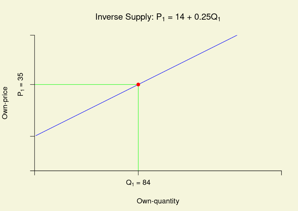
Like the demand schedule, the supply schedule is affected by other variables – supply shifters – that characterize the economics of the production environment. Because market supply arises from the actions of individual agents (firms or producers) who seek to maximize profit, anything that affects cost of production or the potential for profit in alternative production endeavors will impact the relationship between the price and the quantity supplied. Variables that shift the supply schedule will be covered in some depth below. An example of a supply schedule is presented in Figure 1. Aside from the fact that the supply schedule has a positive slope, it is analogous to the demand schedule in that it plots out the schedule of quantity supplied to the market at corresponding own-price levels holding all other variables constant.
Figure \(\PageIndex{1}\): The supply schedule shows the relationship between own-price and own-quantity supplied to the market.
The law of supply states that as price increases, quantity supplied increases and vice versa. Consequently, the supply schedule shows a positive relationship between the market price and amount supplied. The law of supply is the result of two key features of the production environment:
The entry of new firms to the marketplace and the exit of existing firms is determined, in part, by price levels. In the standard economic model, the firm takes inputs such as labor, physical capital, raw materials, and know-how and converts them into a good or service that is sold on the market. All of these inputs come at a cost. A firm will not engage in a production activity unless it is economically feasible. That is, the production activity must generate enough revenue to cover its cost. All else equal, as the price of the good or service rises, it is more likely that new firms will find it feasible to enter the market and produce the good or service at a profit. These new firms will cause the quantity placed on the market to increase. Conversely, as the price of a good or service falls, firms that are presently in the market will find it more difficult to generate a profit and some will go out of business. As these firms leave, the total quantity that is placed on the market declines.
Production processes are generally characterized by the law of diminishing marginal productivity. This means that in order to induce existing producers to put more on the market, the price will need to be high enough to justify bringing less productive and/or more costly resources into production. Most human activities reflect the law of diminishing marginal productivity. In fact, you confront this law as a student. Suppose you spend four hours studying the night before a difficult exam. If you are like most people, the first hour of solid study will be quite a bit more productive than the fourth. By the fourth hour, your are mentally tired, apt to confuse ideas and associations, and are just plain sick of the subject. The same thing holds true in the production of goods and services. The additional inputs that are needed to expand production may be available only in lower quality or accessible only at higher cost. The law of diminishing marginal productivity suggests that cost per unit of output will rise as more output is produced. Consequently, firms will place more output on the market only if a higher price justifies the higher cost of production. This is another reason for the law of supply.