2.3: Profit Maximization for a Price Taking Firm

Supply reflects profit maximizing behavior of firms in the market. The assumption is that firms are in business to make a profit. Profit is composed of two terms. The first is revenue (total sales), and the second is cost (the total cost of doing business). The basic equation for profit is as follows:

\(Profit = Total \: Revenue - Total \: Cost \)

The Price-Taking Assumption

To keep things simple, assume that the market consists of price-taking firms. The price-taking assumption means that any given firm can produce and sell all that it wants at the going market price. This assumption is reasonable if the following two conditions are met.

1. The firm is small relative to the size of the market. The firm must be sufficiently small that its output decisions have a negligible impact on market price. For example, the wheat market is large relative to the size of a given wheat farmer. Even a large farm, with several thousand acres, will have an immeasurable impact on the overall market price. On the other hand, producers of pectin (a food ingredient) are large relative to the size of their market. If one of the major pectin producers opens a new plant or closes an existing plant, there would be an affect on the market price. The assumption of price taking behavior is reasonable for a wheat farm but is unreasonable for a major producer of pectin.
2. The firm’s product or service is indistinguishable from that of other firms. If the assumption of price-taking behavior is valid, then the firm’s output cannot be unique in a manner that enables it to command a premium in the marketplace relative to the products of other firms. This does not entirely rule out quality differences among firms and associated price premiums or discounts for quality attributes. However, quality attributes must be objective and readily identifiable so that products can be sorted into lots of uniform quality. For example, many agricultural commodities are graded by quality. Market prices reflect the quality grade. In these cases, it is the presence of the quality attribute that matters, not the firm that is producing the product. When subjective quality attributes are important to consumers and are conveyed through a brand name or by the reputation of the firm, then the firm is not a price taker.

Why the price-taking assumption? Clearly, the price-taking assumption does not hold in many cases that are interesting and important to understanding the food marketing system. Later in the course, you will consider cases where this assumption does not hold. For now, the assumption enables us to more easily motivate and explore some important economic considerations that relate to the supply side of the market.

Revenue for a Price-Taking Firm

Let \(q\) represent the quantity the firm places on the market. A lower-case \(q\) is used to indicate that this is the firm’s quantity and not the total market quantity (\(Q\)). Total revenue (\(R\)) for the firm is its quantity multiplied by the market price (\(P\)). The price-taking assumption means that the firm can place more on the market without affecting the market price. Its quantity is so small relative to the market quantity that one can assert that \(P\) is not a function of the firm’s quantity (\(q\)), even though \(P\) is a function of the market quantity (\(Q\)). With this in mind, the total revenue for the firm is

\(R = q \times P \)

Because of the price-taking assumption, an output choice only affects revenue through the volume sold. This simplifies the computation of marginal revenue (\(MR\)) and average revenue (\(AR\)) for the firm. Marginal revenue is the change in revenue given a small change in output produced by the firm:

\(MR = \dfrac{\Delta R}{\Delta q} = P\)

where \Delta (capital Greek letter delta) is the change operator. To give you some intuition about \(MR\), note that the total revenue function is a line. The intercept is zero and the slope term (what you learned in algebra as the rise, \(\Delta R\), over the run \(\Delta q\) ) is \(P\).

Average revenue is total revenue divided by the firm’s quantity. In the case of a price-taking firm,

\(AR = \dfrac{R}{q} = \dfrac{q \times P}{q} = P\).

Two points are worth mentioning here. First, given an industry comprised of price-taking firms, both marginal revenue and average revenue for the firm are equal to the market price (\(MR = AR = P\)). Second, because all firms face the market price, all firms have the same marginal revenue and average revenue even if there are differences in technology or ability among the firms.

The Cost Side of Profit

Let us start with some general facts about production cost.

1. Total cost is an increasing function of \(q\). As the volume produced and sold increases, total cost will increase. This reflects the fact that something cannot be produced out of thin air. Production requires inputs (raw materials, labor, capital, etc.). These inputs cost money. As more output is produced, more inputs are required, and production cost will rise accordingly. Sometimes it is said that large firms have lower costs than small firms. It is possible that a large firm could have a lower cost per unit than a small firm, but in this case, the statement is about average cost (cost per unit) and not total cost. Assuming that firms are operating efficiently for their size, then total cost for firms at a larger scale of production will be higher than total cost for firms at a smaller scale.
2. Total cost is an increasing function in input prices. Because production requires inputs, total cost will depend on the prices of inputs. For example, if fertilizer, petroleum, or wage rates increase (decrease), then the cost of producing a given crop will increase (decrease) even if the number of units produced or acres in production remains the same.
3. Total cost reflects efficient use of the prevailing production technology. The firm cannot be maximizing its profit unless it is simultaneously minimizing the cost of producing the profit maximizing output level. Minimizing cost requires that there be no waste in inputs, and the firm is converting inputs into outputs in the best way possible given the technology that is has available. Improvements in technology affect this conversion and impact the production cost. In agriculture, improvements in machinery, genetics, and pest control methods could all be classified as improvements in technology. Such technological improvements usually mean that more output can be produced for a given set of inputs. Stated another way, a technological improvement means that any fixed level of output can be produced with fewer inputs.
4. Cost is an “economic” as opposed to an “accounting” construct. What this means is that the returns that could have been received in alternative production activities are included as an opportunity cost of engaging in the current activity. For example, a farmer who plants corn forgoes the returns that could have been made if an alternative crop were planted instead. The degree of risk inherent in a production activity is also important to the idea of opportunity cost. As a general rule, more-risky activities require higher returns to attract investment of inputs and effort. As risk increases, other, less-risky activities become more attractive. This increases the opportunity cost of staying in the now-more-risky activity.

For simplicity cost will often be expressed only as a function of \(q\) or

\(Total \: Cost = c(q)\)

Total cost depends on all of items 1 - 4 above, so it is a bit of a simplification to only include qq as an argument to the function. In making this simplification, the function shows the relationship between cost and quantity for a fixed technology, a fixed vector of input prices, and constant opportunity cost. Should one or more of these things change, our cost function would shift to reflect the new input prices, new technology, or different opportunity cost. Of course, when necessary, input prices and other items will be included in the cost function. This will be the case later in the chapter.

Marginal and Average Costs

As in the case of revenue, marginal and average concepts on the cost side are of interest as well. Marginal cost (MCMC) is the change in cost resulting from a small change in quantity produced:

\(MC = \dfrac{\Delta c(q)}{\Delta q} = \dfrac{\Delta c(q + \Delta q) - c(q)}{\Delta q} \> 0\).

Marginal cost is strictly positive reflecting the fact that something cannot be produced from nothing. Moreover, an assumption that marginal cost is an increasing function of quantity will often be appropriate. An increasing marginal cost reflects the law of diminishing marginal productivity. Again, this law states that as the producer adds more of any given input, that input’s contribution to output (while positive) diminishes. Average total cost, \(AC\), is defined as the total cost per unit of output:

\(AC = \dfrac{c(q)}{q}\).

Fixed and Variable Costs in the Short Run

In the short run, some cost items may be unavoidable and independent of production. That is, the firm would incur some cost whether or not it actually produces anything and regardless of whether it produces a little or a lot. In these cases, total cost can be expressed as

\(c(q) = f + v(q)\),

where \(f\) is the fixed cost, that portion of total cost which is independent of quantity in the short-run, and \(v(q)\) is the variable cost, that portion of total cost which increases (decreases) as short-run quantity increases (decreases). With this in mind, average total cost can be decomposed into average fixed cost and average variable cost as follows:

\(AC = \dfrac{f}{q} + \dfrac{v(q)}{q} = AFC + AVC\).

AC=fq+v(q)q=AFC+AVC.AC=fq+v(q)q=AFC+AVC.

Earlier it was mentioned that total cost was an increasing function of \(q\), and that this is due to the fact that one cannot produce something from nothing. However, the equation above suggests that average cost could actually decrease as \(q\) increases. You can see this from the two terms that comprise the equation above. The first term, \(AFC= \dfrac{f}{q}\), declines as \(q\) increases. This is because \(q\) is in the denominator. The second term, \(AVC=\dfrac{v(q)}{q}\) may increase or decrease as \(q\) increases. It is always true that \(v(q)\) increases as \(q\) increases because more inputs are needed to produce more output. However, \(q\) is also in the denominator of \(AVC\) making the overall sign of the change with respect to \(q\) ambiguous.

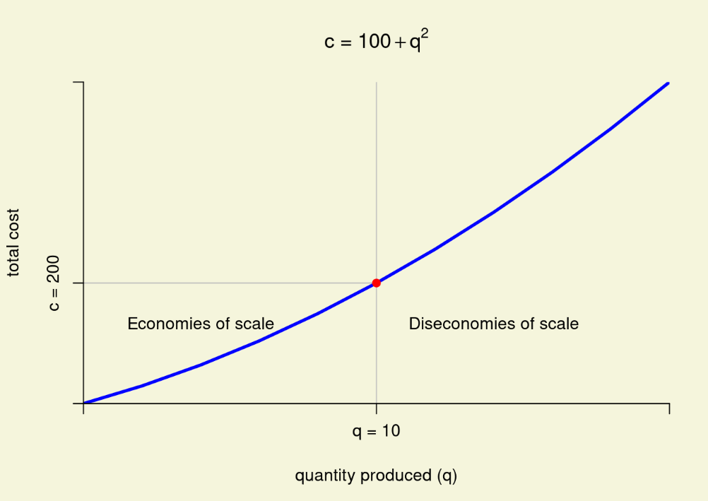
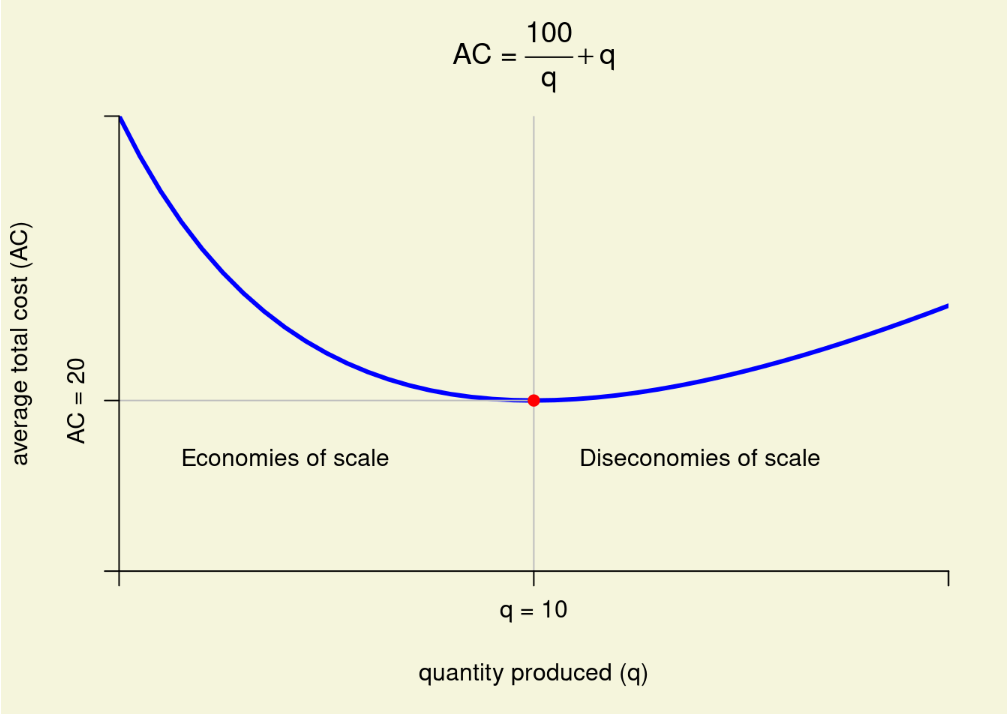
At this point, it should be clear that there are situations where \(AC\) falls as more output is produced. When this is true, there are economies of scale. Conversely, when \(AC\) increases as \(q\) increases, there are diseconomies of scale. Figure \(\PageIndex{2}\) presents a cost function that exhibits both economies and diseconomies of scale over different ranges of output. In the figure, the firm is operating under economies of scale at output levels below \(q=10\) and under diseconomies of scale at output levels greater than \(q=10\). Notice from Panel A of Figure \(\PageIndex{2}\) that cost always increases as output increases. Panel B, however, shows that average cost declines until the firm reaches an output of 10 units and then increases afterwards. Note that the firm faces fixed cost of \(f = 100\) and variable cost of \(v(q) = q^{2}\). The corresponding \(AFC\) and \(AVC\) are \(AFC = frac{100}{q}\) and \(AVC = q\), respectively. The reason for the economies of scale is that at output levels below \(q = 10\), \(AFC\) is declining at a faster rate than \(AVC\) is increasing. At output levels greater than \(q = 10\), \(AFC\) continues to decline but at a lower rate than \(AVC\) increases.

Panel A: Total cost.

Panel B: Average cost.

Figure \(\PageIndex{2}\): Illustration of total cost and average cost with ranges of output showing economies and diseconomies of scale.

Later in the course, you will see that economies of scale are important to coordination as products move through different stages of the vertical chain. Specifically, the decision of whether to source a supply or service through the market or internally through vertical integration depends to large extent on whether the firm’s demand for the input is large enough to justify operation at an efficient scale. For now, however, the goal is to emphasize the difference between total and average cost and their relevance to the law of supply. Let us turn our attention to this topic.

The Producer’s Decision to Enter, Remain, or Exit the Market

One reason for the law of supply lies in decisions by producers to enter or exit the market. The supply side of the market will attract entrants whenever a producer sees that \(P \geq AC\). Remember that \(AC\) includes opportunity cost, so \(P \>AC\) means that the producer’s profit margin in this market is better than alternative production activities available to him or her. As the market price rises, more producers will see that \(P \> AC\) and will enter the market. Additional entry into the market at higher prices causes more output will be placed on the market. Exactly what the law of supply says will happen.

The converse is also true, as the market price falls, some producers will exit the market. However, the price at which producers exit the market will often be lower than average total cost. In fact, it could be much lower as you will see in the vineyard example below. The reason for this lies in the fact that over some planning horizons, average total cost includes a portion that is fixed. The producer incurs the fixed cost in the short run regardless of whether he or she produces anything. If the producer exits the market, the short-run loss will be equal to the fixed cost. If the producer remains in the market, loss could be reduced provided the market price is high enough to cover the variable cost. There are three price points that are important to the entry and exit decision.

1. The break-even price point is \(P = AC\). When the market price exceeds the break-even point, the market will attract new entrants.
2. The shutdown price point is \(P = AVC\). At a price below the shut-down point, the firm will lose less by exiting the market. The short-run loss will be equal to the firm’s fixed cost.
3. A firm will remain in the market and continue to operate when the market price is between the break-even and shutdown points, \(AVC \< P \< AC\)

The difference between the break-even and shutdown points results from differences in the length of run. In the long run, all cost items are variable. In the equation for average total cost above, \(f=0\) and so \(AC = AVC\). In other words, there is no difference between the break-even and shutdown points in the long run. In the short run, however, some cost items cannot be avoided and must be incurred regardless of whether the firm operates. For example, suppose the firm has a long-term lease on a production facility. In the short run, the lease must be paid regardless of whether the firm operates. The cost of the lease is fixed. The short run is the length of time it would take the firm extricate itself from the lease obligation.

Vineyard Economics: A Case Example

Production of grapes involves a large fixed cost in terms of a trellis system to support the grape vines, a drip irrigation system to deliver water and nutrients to the vineyard, and expenses incurred to establish a productive vineyard, a process that takes several years. Consider some wine-grape production budgets published for the Finger Lakes region of New York (White 2011). Here is a direct link: download from ageconsearch.umn.edu. Although it would be a good idea to review other parts of the publication for background, the focus will be specifically on Table 11 of the publication. White’s (2011) budgets are chosen since they are quite detailed, provide a good overview of what it takes to establish a vineyard, and are representative of Eastern viticulture regions. With the exception of Pinot Noir, the varieties that White (2011) considers can be raised in regions of Arkansas suitable for the production of bunch grapes (see Noguera et al. 2005). As you peruse White’s (2011) budget publication, consider the following:

1. How has the author handled the issue of “economic” versus “accounting” cost? Can you provide some examples of cost items included in the budget that would indicate that the author is attempting to measure economic costs? If so, what?
2. Why did the author classify some costs as fixed and others as variable? Is there any feature that all fixed costs have in common? What do all variable costs have in common?
3. How did the author compute the break-even price? You should take a moment to compute the average fixed cost ($/ton) and average variable cost ($/ton) assuming the yield targets reported in the top row of Table 11.
4. Given the values reported in Table 11, would you expect to see new vineyards being established? Why or why not?
5. Assuming that variable costs and yield targets reported in Table 11 are typical for vineyards that have already been established, do you expect existing vineyards to shut down in the short run? Why or why not?
6. What is the potential length of the short run in a vineyard operation? How long does the author assume the vineyard will be productive once it has been established?

Demonstration 1 is calibrated to match the last column of Table 11 in White (2011). This is the column for Riesling grapes. In the demonstration, quantity is 3.4 tons/acre if the vineyard continues operations. Otherwise, quantity is zero. One thing to notice is the high fixed cost of the Riesling vineyard. Total fixed cost is $2,445 per acre. Dividing this by tons produced indicates an average fixed cost of $719 per ton. In the demonstration, this $719 is the difference between the break-even threshold (solid blue line) and the shutdown threshold (solid red line). When Demonstration 1 first loads, it matches the assumptions of White (2011) and shows a market price of $1,300 per ton, average variable cost of $817 per ton, and an $803 loss per acre on the Riesling vineyard. If it does not match, you can reload the page so that it will.

The first thing to point out is that at the price of $1,300, the vineyard is not profitable. It cannot cover its total cost comprised of both its fixed and variable cost. Nevertheless, you would expect a vineyard in this situation to continue operations since $1,300 is well above the shutdown point of $817. The table in the demonstration shows two scenarios. If the vineyard continues to operate at a price of $1,300 per ton it loses $803 per acre. If it shuts down at this price, it loses $2,445 per acre. Clearly, its best choice is to continue operations at a price of $1,300 per ton. However, this price will not attract any new vineyards into the market.

In the demonstration, you can control two things: the market price and the magnitude of average variable costs. Whenever the market price is above the blue, break-even threshold, you would expect entrants into Riesling vineyards. Whenever, price falls below the red, shutdown threshold, you would expect existing Riesling vineyards to exit. Notice that the market price affects the entry/exit decision as does the magnitude of average variable cost.

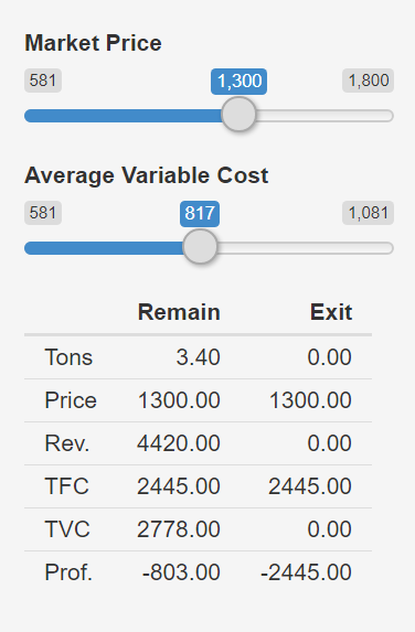
Demonstration \(\PageIndex{1}\): The decision to enter, exit or remain.

There are three takeaways from the entry and exit decision as explained here. The first is simply that producers enter the market if the price exceeds their break-even point, remain in the market when the price is between the break-even and shutdown points, and exit the market if price falls below the shutdown point. This entry and exit decision is one reason for the law of supply.

The second takeaway is that supply can be fixed in the short run, and, as the vineyard example demonstrates, the short run could be a long time. Thus, in some markets, there can be stickiness in supply because it will take a large increase or decrease in prices to trigger the entry or exit decision. As you will learn later in the course, this can give rise to cyclical patterns in agricultural prices.

The third takeaway is a bit more subtle but is important for the organization of agricultural markets. Imagine that you are the owner of a Riesling vineyard similar to the one in the example above. Now suppose that you have a limited number of buyers for your grapes. From a marketing standpoint, the overarching concern is that once your vineyard is established, a buyer may be able to extract substantial price concessions from you. This is possible because of the large difference between the break-even and shutdown price. There is little concern if you have many alternative buyers, but when the number of buyers is small, the potential for opportunistic behavior may prevent an open market from functioning. Coordination of supply with demand could still take place but would involve formal or implicit contracts. In some cases, independent suppliers may be so concerned about opportunistic behavior on the part of the buyer that they will not enter the market. The buyer will need to backward integrate in order to secure the supplies. Many wineries are, in fact, backward integrated into vineyard operations.

Profit Maximization

In the vineyard example, the firm’s quantity choice was binary in that the vineyard either continued to operate or it shutdown. If the vineyard continued to produce, its output was 3.4 tons/acre, give or take a bit. This is because yield is related to quality of the grapes (and their value to wineries). Moreover, a vineyard has a more or less fixed capacity once it has been established. The quantity choice is much less binary in many other production settings. For instance, I worked in the box cooler of a beef packing plant when I was younger. The packing plant could increase the volume of cattle it processed if it was profitable for it do so. In these situations, I worked longer hours and/or weekend shifts. The plant paid overtime in these situations, which was time and a half. Thus, the plant could increase its output but only at a higher cost. Labor was the plant’s second highest cost item after cattle.

The firm’s profit is maximized when marginal revenue equals marginal cost. This condition is \(P = MR = MC\) in the case of a price taking firm. The logic supporting this condition is as follows:

1. Suppose that \(P \> MC\) at some output level \(q = \tilde{q}\). In this situation, the firm could increase its output by \(\Delta q\), a small amount. Its revenue would go up by \(P\), but its cost would only go up by \(MC \< P\). For this reason, its profit will go up if it produces \(Delta q\) more units. Hence, \(q = \tilde{q}\) could not be a profit maximizing level of quantity if \(P \> MC\) because there is another value of \(q\), namely \(q = \tilde{q} + \Delta q\), that provides a higher level of profit than \(q = \tilde{q}\).
2. Suppose instead that \(P \<MC\) at some output level \(q = \tilde{q}\). In this situation, the firm could decrease its output by \(\Delta q\), a small amount. Its revenue would go down by \(P\), but its cost would go down by \(MC \> P\). Its cost savings from reducing its output by \(\Delta q\) would more than offset its revenue loss. Overall profit would go up. Hence, \(q = \tilde{q}\) could not be a profit maximizing level of quantity if \(P \< MC\) because there is another value of \(q\), namely \(q = \tilde{q} - \Delta {q}\), that provides a higher level of profit than \(q = \tilde{q}\).

This logic suggests that the only way for \(q = \tilde{q}\) to be a profit maximizing level of output is if marginal cost at \(q = \tilde{q}\) is equal to the price. The beef packing plant I worked for understood this concept. When boxed beef prices justified the overtime costs, it meant that \(P\) was greater than \(MC\), and the company had me work longer hours and/or weekend shifts. Conversely, when \(P\) was less than \(MC\), my overtime hours were cut back.

For a price-taking firm, the condition \(P = MC\) defines the individual firm’s supply schedule. As the output price increases, producers will find it profitable to produce more units (albeit at higher marginal cost). This relationship holds in the short run so long as the market price is above the shutdown point (\(P \> AVC\)). Use Demonstration \(\PageIndex{2}\) below to gain some intuition about this. In the demonstration, the shaded rectangular area represents the size of the firm’s profit (if blue) or loss (if red). Notice in the demonstration that when you choose the quantity that equates the firm’s marginal cost with the market price, you cause this rectangular area to be maximized if blue or minimized if red. Change the price in the demonstration. Then adjust the quantity to maximize profit. You will see that the firm should expand or reduce its output to maximize its profit if price increases or decreases.

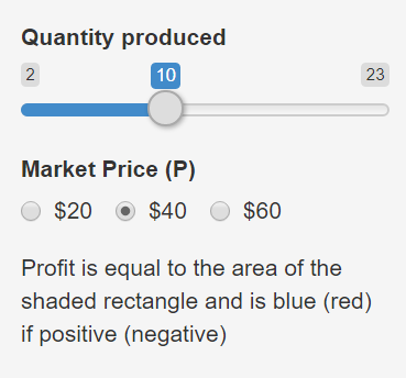
Marginal Cost (MC) = $40.00

Average Total Cost (AC) = $30.00

Profit = (AR - AC)q =$100.00

Demonstration \(\PageIndex{2}\): The firm’s problem when \(C(q) = 100 + 2q^{2}\).