Several factors affect the magnitude of the own price elasticity. Knowing these factors can help you make a determination about the likely range of an elasticity in cases where you lack the data needed to estimate it precisely.
Share of Income Devoted to the Product
As a general rule, demand will be more elastic the larger the share of the consumer’s budget required to purchase the item. The rationale here is that the consumer will be more likely to shop around, wait for discounts, or delay making making large purchases until necessary. Demand tends to be more elastic because the consumer stands to capture a large dollar value of additional surplus if he or she can find a better price.
Availability of Substitutes
When substitute products are readily available, demand will be more elastic. Remember from Chapter 1 that two phenomena underpin the law of demand. First, when the price increases, consumers who continue to purchase the product will purchase less. This is a result of the law of diminishing marginal utility. Second, some consumers drop out of the market altogether because participation in this market will no longer provide them with an opportunity for positive consumer surplus at the higher price. When substitute products are readily available, the defection of consumers to lower priced alternatives becomes the driving factor and makes demand very responsive to price changes.
Length of Run
Demand will be more elastic in the long run. The rationale here is that as time passes, consumers have more opportunities to adjust their consumption behavior. One way to model demand over time is to specify quantity demanded in the current time period (period t) as a function of quantity demanded the period before (period t-1). In this case, demand in the short run can be expressed as
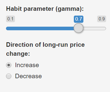
where \(\alpha > 0\), \(\beta < 0\), and \(0 \leq \gamma < 1\). In this equation, \(\gamma\), the Greek letter gamma, is a habit parameter. As \(\gamma\) approaches one, habit formation is very strong and consumption in prior periods has a large impact on consumption today. Moreover, when \(\gamma\) is close to one, it will take many periods to converge to the new long-run demand. Demonstration \(\PageIndex{1}\) is designed to help you see this. In the demonstration, you can vary the habit parameter to see the time it takes to adjust from one long-run quantity to another. When the habit parameter is small, adjustment takes place rapidly. When it is large, complete adjustment takes much longer.
Demonstration 4. The habit parameter affects the time to converge to a new point on the long-run demand schedule.
In the long-run, demand at time \(t\) will converge to demand at time \((t-1)\). With this in mind, one can set \(Q_{1}^{LR} = Q_{1}^{t} = Q_{1}^{t-1}\) in the short run demand equation and solve for \(Q_{1}^{LR}\) to get long-run demand as
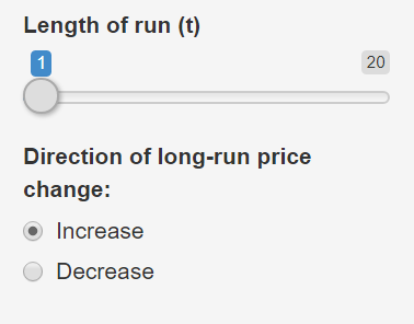
Demonstration \(\PageIndex{2}\), shows the convergence process as time passes. Note that as time goes on, the effect of \(Q_{1}^{t=0}\) becomes less and less until it disappears completely. This is an asymptotic process so you do not see complete convergence in the 20 periods represented below. Nevertheless, after 20 periods, there is very little difference between the short-run and long-run demands. You should also be able to verify from Demonstration \(\PageIndex{2}\) that demand is more elastic in the long run than in the short run.
Demonstration \(\PageIndex{2}\). Convergence to long-run demand over time.
Demand at Different Stages of the Market
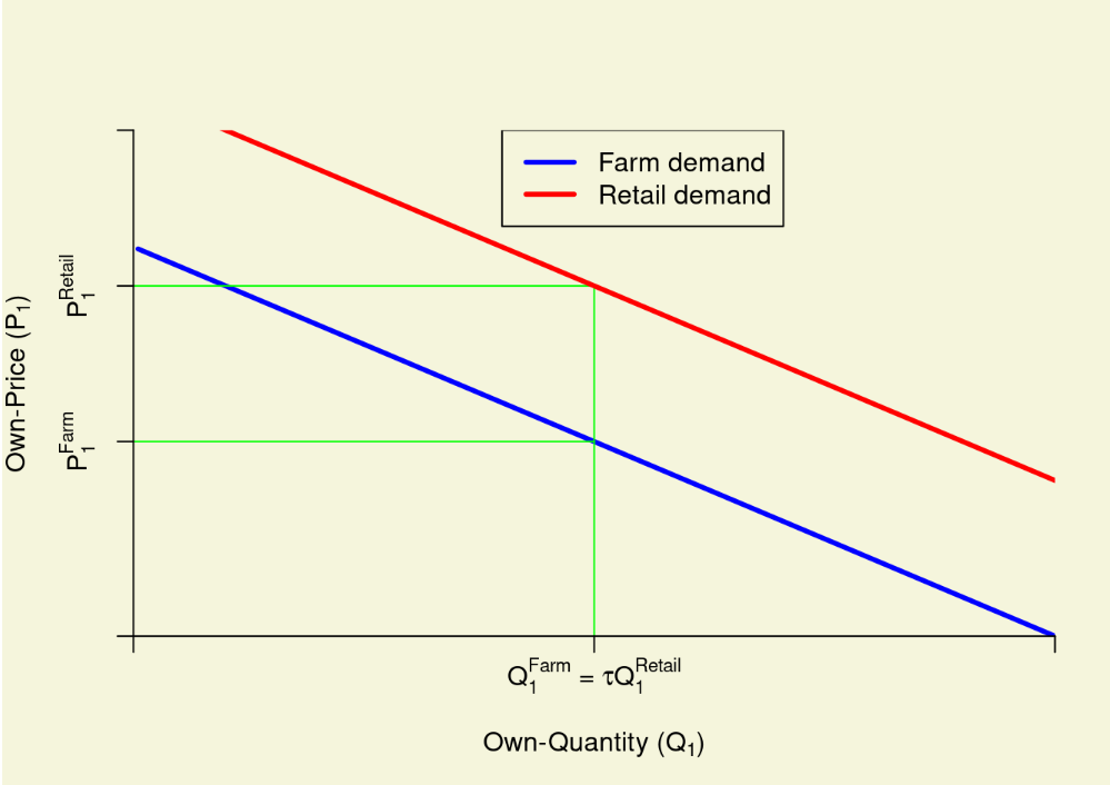
Many retail food products require fixed proportions of farm products. For example, a pint of blueberries at the retail level requires a pint of blueberries from the farm. A few pints will be damaged in transit from the farm to retail and so offering a certain quantity of blueberries on the retail market may be some fixed proportion ττ of the number of pints from the farm, and ττ may not be equal to one. Nevertheless, there is a clear relationship between the quantity of the farm and retail product. If the assumption of fixed proportions applies, one can express the farm and retail product on the same quantity axis as is done below in Figure \(\PageIndex{1}\).
Figure \(\PageIndex{1}\) shows demand at the farm level and the retail level. The vertical difference between these two demand schedules represents the cost of getting the product from farm to retail. In the case of blueberries, these costs would include things like shipping and stocking. If these costs are independent of the quantity of the farm product being offered for sale at retail, the farm-to-retail markup will be constant. This means that the farm demand will be parallel to the retail demand. This is also shown below in Figure \(\PageIndex{1}\).
What does any of this have to do with elasticity? Well, it can be shown that under certain conditions, the farm demand will be less elastic than the retail demand. Note that the farm and retail demand schedules have the same slope. Let \(\beta < 0\) represent this slope. Also note that \(Q_{1}^{Farm} = \tau Q_{1}^{Retail}\). Using the point formula one can see that \(0 > \beta \times \dfrac{P_{1}^{Farm}}{Q_{1}^{Farm}} > \beta \times \dfrac{P_{1}^{Retail}}{\tau Q_{1}^{Retail}}.\)
In other words, \(0 > \epsilon_{11}^{Farm} > \epsilon_{11}^{Retail}\) farm demand is less elastic than retail demand.
Figure \(\PageIndex{1}\): Elasticity at different points in the supply chain.