In a market, demand and supply come together to determine the price and quantity of a product. A market is said to be in equilibrium when the prevailing price causes the quantity supplied to equal the quantity demanded. The term equilibrium suggests a point of stability. Because supply equals demand at an equilibrium, there is no reason for consumers to bid prices up through unmet requests for the product nor is their a reason for producers to bid prices down because of untaken offers of the product. Price is, in this respect, stable.
Consider an example involving a single market. Suppose that the demand for good 1 is given by
\(Q_{1}^{D} = 100 - \dfrac{1}{2} P_{1} + D,\)
where \(Q_{1}^{D}\) is quantity demanded, \(P_{1}\) is price, and \(D\) is a demand shock. \(D\) can be positive, negative, or zero.
Next, suppose that supply for good 1 is given by
\(Q_{1}^{S} = -20 + P_{1} + S,\)
where \(Q_{1}^{S}\) is quantity supplied and \(S\) is a supply shock. Again, \(S\) can be positive, negative, or zero.
To find the equilibrium price, set \(Q_{1}^{S} = Q_{1}^{D}\) and solve for \(P_{1}\) as follows:
\(-20 + P_{1} + S = 100 - \dfrac{1}{2}P_{1} + D \Rightarrow P_{1} = 80 + \dfrac{2}{3}(D-S).\)
Next, substitute this solution for \(P_{1}\) into the supply or the demand equation. If the solution for \(P_{1}\) is correct, you will get the same quantity regardless of which equation you use:
\(Q_{1}^{S} = -20 + 80 + \dfrac{2(D-S)}{3} + S = 60 + \dfrac{2D+S}{3}.\)
\(Q_{1}^{D} = 100 - \dfrac{1}{2}(80 + \dfrac{2(D-S)}{3}) + X = 60 + \dfrac{2D+S}{3}.\)
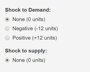
An equilibrium based on this example is depicted below in Demonstrations \(\PageIndex{1}\) and \(\PageIndex{2}\). Note that when there is no demand or supply shock (\(D = S = 0\)), \(P_{1}^{E} =80 \: and \: Q_{1}^{E} = 60\). This is the initial equilibrium depicted in the demonstrations. Use Demonstration \(\PageIndex{1}\) to add a positive shock to demand. When you do this, the demand schedule shifts to the right by 12 units. This disrupts the equilibrium. At the current price of $80, only 60 units are supplied but now 72 units would be demanded. Since demand now exceeds supply, the price will be bid up until a new equilibrium price of $88 is reached which causes the new demand schedule to equate with the supply schedule at a new equilibrium quantity of 68 units. Thus, the initial shock of positive 12 units ultimately resulted in an 8 unit increase in the equilibrium quantity after the market price adjusted to a new equilibrium price.
Reset the demand shock in Demonstration \(\PageIndex{1}\) to be zero. You will return to the original equilibrium of \(P_{1}^{E} = 80 \: and \: Q_{1}^{E} = 60\). Now use the demonstration to apply a negative shock to demand. This causes demand to shift to the left by 12 units. At the current price of $80, only 48 units would be demanded after the shock, but suppliers will continue to offer 60 units on the market. Because supply now exceeds demand, the price will be bid down until the market reaches a new equilibrium price of $72 and a new equilibrium quantity of 52 units. Again the initial shock of negative 12 units ultimately resulted in an 8 unit decrease in the equilibrium quantity after the market price reached a new equilibrium.
Demonstration \(\PageIndex{1}\). An Equilibrium and equilibrium adjustment resulting from a demand shock.

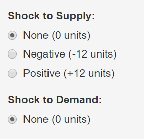
Demonstration \(\PageIndex{2}\), is similar except that it allows you to consider the effect of positive or negative shocks to supply as opposed to demand. Spend some time with demonstration \(\PageIndex{2}\) to visualize the effects of a positive or negative supply shock. As you do, note that a shock disrupts the equilibrium so that supply no longer equals demand. As a result, prices are bid up or down as necessary until a new equilibrium price is determined that matches demand to the new supply schedule. Pay attention to the direction of the quantity and price change in response to the positive and negative supply shocks.
Demonstration \(\PageIndex{2}\). An equilibrium and equilibrium adjustment resulting from a supply shock.
Exogenous and Endogenous Variables in an Equilibrium Model
In the above example, an equilibrium was found by solving a system of equations. In the case of one market, there are two equations (one supply equation and one demand equation) and two unknowns (the equilibrium price and the equilibrium quantity). These unknown variables are called endogenous variables. They are given this name because they are determined inside the system of equations. The etymology of the prefix “endo” is from a Greek word meaning “within.” In general, the number of endogenous variables in the system will be equal to the number of demand and supply equations. For example, in a model of two markets, there are four equations (two pairs of demand and supply equations) and four endogenous variables (an equilibrium price and quantity in each of the two markets).
Exogenous variables affect the equilibrium but are determined outside of the system of equations. As you might have guessed, the prefix “exo” also has its origin in a Greek word meaning “outside.” In terms of the demand or supply schedules, a change in an exogenous variable causes one or more of the schedules to shift. In the example above, there were two exogenous variables: \(D\) and \(S\). There is no upper limit on the number of exogenous variables that can be included in the system. Exogenous variables will be a subset of those designated in chapters 1 and 2 as demand or supply shift variables. However the term “shifter” and “exogenous” are not synonymous. To be truly exogenous, the shift variable needs to be unaffected by the markets being analyzed in the model. Otherwise, it is not truly exogenous. For example, one could argue that beef and pork are substitutes. If this is true, the price of pork shifts the demand for beef. Nevertheless, it would problematic to assume that the price of pork is exogenous because the price of beef also shifts the demand for pork. In this case, an accurate model would need to encompass the markets for both beef and pork, in which case the prices and quantities of beef and pork would all be endogenous variables in the model.
In many contexts, a change in average consumer income, another demand shift variable, could be treated as exogenous. This is fine so long as it is reasonable to assert that income is dictated by macroeconomic forces that are minimally affected by the market being analyzed. However, there will be cases where income should not be considered exogenous. In fact, income is endogenous in one of the consumer models that will be presented in Chapter 5. In this model, income is determined by the consumer’s allocation of time spent in leisure activities, in the labor force, and in household production. Similarly, in some cases, the supply side of the market will be small enough to not materially affect the price of an input. In such cases, it may be reasonable to assume that input prices are exogenous variables within the model. In others, it will be necessary to formally incorporate input markets into the model and input prices will be endogenous.
A Basic Framework for Identifying the Cause of an Equilibrium Change
Demonstration \(\PageIndex{3}\). A basic framework for identifying the cause of an equilibrium change.
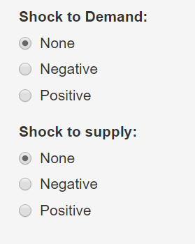

In regions 1 and 3 of Demonstration \(\PageIndex{3}\), you can conclude with certainty that demand has shifted. If the new equilibrium lies to the southwest of the initial equilibrium (the region denoted as 1), then demand has decreased (shifted to the left). If the new equilibrium lies to the northeast of the initial equilibrium (the region denoted as 3), then demand has increased (shifted to the right). If a new equilibrium lies in regions 1 or 3, conclusive statements cannot be made about a supply shift. Supply might have shifted but one cannot be sure. To help you see this, use the demonstration to add a negative shock to demand and a positive shock to supply. The new equilibrium point lies in region 1 even though supply has also shifted. Now set the supply shock back to “none”. The resulting equilibrium is still in region 1. In region 1 all you can say with certainty is that demand has decreased. Supply may or may not have shifted. No conclusive statement can be made about supply if you are in region 1.
In regions 2 and 4 of Demonstration \(\PageIndex{3}\), you know that supply has shifted. If the new equilibrium lies to the northwest of the initial equilibrium (the region denoted as 2), then a conclusive statement can be made that supply has decreased (shifted to the left). If the new equilibrium lies to the southeast of the initial equilibrium (the region denoted as 4), then a conclusive statement can be made that supply has increased (shifted to the right). Again, demand may or may not have shifted if a new equilibrium is observed in regions 2 or 4. However, there is no way for a new equilibrium to be in regions 2 or 4 without there having been a supply shift.
In Demonstration \(\PageIndex{3}\), you can see the demand and supply schedules. However, the conclusions above can be inferred from this basic framework even if you could not. The framework requires only that the laws of demand and supply apply to the market being examined. Use Demonstration \(\PageIndex{3}\) to verify the conclusions summarized in Table \(\PageIndex{1}\). Because you are given example demand and supply schedules in Demonstration \(\PageIndex{3}\), you may question why some of the directions are marked as ambiguous in the table. For example, a positive demand shock and negative supply shock results in a slight increase in equilibrium quantity given the example schedules in the demonstration. However, another set of example schedules could have been provided that would have shown a decrease in quantity. Note that the ambiguous cases in table \(\PageIndex{1}\) happen when demand and supply change simultaneously and when the impact of the demand and supply changes on price or quantity offset one another. The actual change in these ambiguous cases depends on the magnitude of the supply shock relative to the demand shock and, as you will see momentarily, on the elasticity of demand and supply.
Table \(\PageIndex{1}\). Effects of demand and supply shocks on a market equilibrium
| Supply Shock |
Demand Shock |
Effect on Eq. Price |
Effect on Eq. Quantity |
| + |
None |
↓ |
↑ |
| − |
None |
↑ |
↓ |
| None |
+ |
↑ |
↑ |
| None |
− |
↓ |
↓ |
| + |
+ |
Ambiguous |
↑ |
| + |
− |
↓ |
Ambiguous |
| − |
+ |
↑ |
Ambiguous |
| − |
− |
Ambiguous |
↓ |

