In a model with a single market, there are two endogenous variables and two equations. You can find a unique solution for \(\% \Delta P\) and \(\% \Delta Q\). With multiple markets, there will be two equations (one supply equation and one demand equation) for each market. Solving for the endogenous variables becomes a bit messy unless you use matrix algebra. Let us step through the process of putting a two-market model, such as those depicted in Demonstrations 4.4.1 and 4.4.2 above, into matrix format. In the case of two markets there will be four equations.
\(Supply \: in \: Market \: 1: \% \Delta Q_{1} = \phi_{11} \% \Delta P_{1} + \phi_{12} \% \Delta P_{2} + \% \Delta S_{1}\)
\(Demand \: in \: Market \: 1: \% \Delta Q_{1} = \varepsilon_{11} \% \Delta P_{1} + \varepsilon_{12} \% \Delta P_{2} + \% \Delta D_{1}\)
\(Supply \: in \: Market \: 2: \% \Delta Q_{2} = \phi_{21} \% \Delta P_{1} + \phi_{22} \% \Delta P_{2} + \% \Delta S_{2}\)
\(Demand \: in \: Market \: 2: \% \Delta Q_{2} = \varepsilon_{21} \% \Delta P_{1} + \varepsilon_{22} \% \Delta P_{2} + \% \Delta D_{2}\)
To express these equations in matrix notation, it is first necessary to make sure terms in these equations are arranged appropriately
- First, get all the endogenous variables on the left side of the equations and all the exogenous terms on the right. There are four endogenous variables in this system. They are \(\% \Delta Q_{1}\), \(\% \Delta Q_{2}\), \(\% \Delta P_{1}\), and \(\% \Delta P_{2}\). The exogenous terms are \(\% \Delta S_{1}\), \(\% \Delta D_{1}\), \(\% \Delta S_{2}\), and \(\% \Delta D_{2}\).
- Second, there must be place for each endogenous variable in each equation. As shown above, \(\% \Delta Q_{1}\) appears only in the supply and demand curves for Market 1 and \(\% \Delta Q_{2}\) appears only in the supply and demand equations for Market 2. However, you can add \(0 \times \% \Delta Q_{1}\) to the equations to Market 2 and \(0 \times \% \Delta Q_{2}\) to the equations for Market 1 so that each endogenous variable has a place in each equation.
- Finally, each endogenous variable must appear in the same order in each equation.
An arrangement that meets all of these criteria is as follows.
\(Supply \: in \: Market \: 1: \% \Delta Q_{1} + 0 \times \% \Delta Q_{2} - \phi_{11} \% \Delta P_{1} - \phi_{12} \% \Delta P_{2} = \% \Delta S_{1}\)
\(Demand \: in \: Market \: 1: \% \Delta Q_{1} + 0 \times \% \Delta Q_{2} - \varepsilon_{11} \% \Delta P_{1} - \varepsilon_{12} \% \Delta P_{2} = \% \Delta D_{1}\)
\(Supply \: in \: Market \: 2: 0 \times \% \Delta Q_{1} + \% \Delta Q_{2} - \phi_{21} \% \Delta P_{1} - \phi_{22} \% \Delta P_{2} = \% \Delta S_{2}\)
\(Demand \: in \: Market \: 2: 0 \times \% \Delta Q_{1} + \% \Delta Q_{2} - \varepsilon_{21} \% \Delta P_{1} - \varepsilon_{22} \% \Delta P_{2} = \% \Delta D_{2}\)
Notice that each endogenous variable now appears in each equation. In each equation, \(\% \Delta Q_{1}\) appears first, \(\% \Delta Q_{2}\) appears second \(\% \Delta P_{1}\) appears third, and \(\% \Delta P_{2}\) appears fourth. It does not matter which endogenous variable appears first, second, third, or fourth so long as the order of these variables is uniform across all equations. In other words, the variable that appears first must be first in each equation, the variable that appears second must be second in each equation, and so forth. Finally, it does not matter the order of the equations. For example, you could have arranged these equations so that both supply equations were listed first followed by both demand equations, if that was your preference. This system of equations as arranged above can be expressed in matrix form as shown below.
\(\begin{bmatrix} 1 & 0 & -\phi_{11} & -\phi_{12} \\ 1 & 0 & -\varepsilon_{11} & -\varepsilon_{12} \\ 0 & 1 & -\phi_{21} & -\phi_{22} \\ 0 & 1 & -\varepsilon_{21} & -\varepsilon_{22} \end{bmatrix} \: \begin{bmatrix} \% \Delta Q_{1} \\ \% \Delta Q_{2} \\ \% \Delta P_{1} \\ \% \Delta P_{2} \end{bmatrix} = \begin{bmatrix} \% \Delta S_{1} \\ \% \Delta D_{1} \\ \% \Delta S_{2} \\ \% \Delta D_{2} \end{bmatrix}\)
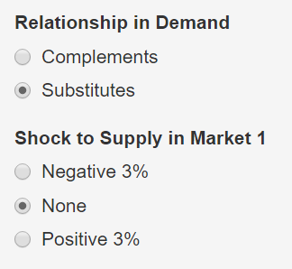
The equations are now in the form \(\bf{Ax = b}\), where \(\bf{A}\) is the matrix containing zeros, ones, and the elasticities of demand and supply; \(\bf{x}\) is the vector of endogenous variables; and \(\bf{b}\) is the vector of exogenous shocks. The solution to this system of equations is given by \(\bf{x = A^{-1}b}\). Demonstration \(\PageIndex{1}\), provides an example of two markets like those in depicted graphically above in Demonstrations 4.4.1 and 4.4.2. The markets in the demonstration are related in demand but not in supply. The demonstration permits you to examine a supply shock in Market 1. Like the demonstration above, you can see the role of feedback from Market 1 to Market 2 when the supply shock occurs. Take a moment to verify that you understand how the matrices in Demonstration \(\PageIndex{1}\) are constructed given the data provided. Notice also that the effects of the supply shock conform to those you analyzed above in Demonstrations 4.4.1 and 4.4.2.
Demonstration \(\PageIndex{1}\). An exogenous supply shock in a two market system. The markets are related in demand but unrelated in supply.
Given the following:
\(\phi_{11} = 1.3; \phi_{12} = 0; \varepsilon_{11} = -1.2; \varepsilon_{12} = 0.5.\)
\(\varepsilon_{21} = 0; \phi_{22} = 0.9; \varepsilon_{21} = 0.6; \varepsilon_{22} = -1.4.\)
The A matrix is:
\(\bf{A} = \begin{bmatrix} 1 & 0 & -\phi_{11} & -\phi_{12} \\ 1 & 0 & -\varepsilon_{11} & -\varepsilon_{12} \\ 0 & 1 & -\phi_{21} & -\phi_{22} \\ 0 & 1 & -\varepsilon_{21} & -varepsilon_{22} \end{bmatrix} = \begin{bmatrix} 1 & 0 & -1.3 & 0 \\ 1 & 0 & 1.2 & -0.5 \\ 0 & 1 & 0 & -0.9 \\ 0 & 1 & -0.6 & 1.4 \end{bmatrix}\)
The b matrix is:
\(\bf{b} = \begin{bmatrix} \% \Delta S_{1} \\ \% \Delta D_{1} \\ \% \Delta S_{2} \\ \% \Delta D_{2} \end{bmatrix} = \begin{bmatrix} 0 \\ 0 \\ 0 \\ 0 \end{bmatrix}\)
The solution matrix (x) is:
\(\bf{x} = \begin{bmatrix} \% \Delta Q_{1} \\ \% \Delta Q_{2} \\ \% \Delta P_{1} \\ \% \Delta P_{2} \end{bmatrix} = \begin{bmatrix} 0 \\ 0 \\ 0 \\ 0 \end{bmatrix} \)
Linear systems of equations can be solved easily with today’s computers. For example, R, the software used to develop An Interactive Text is an excellent package to solve these kinds of systems. Figure \(\PageIndex{1}\) contains the code needed to replicate the results in Demonstration \(\PageIndex{1}\) within an R session. R is a good choice for this kind of work because it is designed to do matrix operations, is open source, and is widely used across industry, government, and academia. The grey blocks in Figure \(\PageIndex{1}\) are the commands you would submit to define the matrices or solve the equations. The white blocks show the output that the R commands would generate. Note that the solution in Figure \(\PageIndex{1}\) matches that in Demonstration \(\PageIndex{1}\) for a positive supply shock when the products are substitutes in consumption.
## The command below defines and prints the A matrix using the elasticities given in Demonstration 6
## (case of substitutes).
A<-matrix(c(1, 0, -1.3,    0,
            1, 0,  1.2, -0.5,
            0, 1,    0, -0.9,
            0, 1, -0.6,  1.4),
          nrow=4,byrow=T,
          dimnames=list(c("S1","D1","S2","D2"),c("Q1","Q2","P1","P2"))
          ); A
##    Q1 Q2   P1   P2
## S1  1  0 -1.3  0.0
## D1  1  0  1.2 -0.5
## S2  0  1  0.0 -0.9
## D2  0  1 -0.6  1.4
## The command below defines and prints the b vector for a positive 3 percent supply shock to Market 1.
b<-matrix(c(3,0,0,0),nrow=4,dimnames=list(c("S1","D1","S2","D2"),c("shock")));b
##    shock
## S1     3
## D1     0
## S2     0
## D2     0
## The command below finds the solution to the system of equations and rounds it to three decimal places.
x<-round(solve(A,b),digits=3)
## The command below formats the row names and column name of the solution vector and displays it.
dimnames(x)<-list(c("Q1","Q2","P1","P2"),c("Pct.Change")); x
##    Pct.Change
## Q1      1.354
## Q2     -0.297
## P1     -1.266
## P2     -0.330
Figure \(\PageIndex{1}\): Using R to find the solution to a two-market equilibrium model.
Most spreadsheets are also capable of solving these kinds of linear systems. LibreOffice Calc is an open-source spreadsheet program that can take the inverse of a block of cells you define as a matrix and multiply it by a column vector thereby implementing the solution to a market equilibrium model as \(\bf{x = A^{-1}}\). The spreadsheet functions needed are minverse(), to take the inverse of the \(\bf{A}\) matrix and mmult(), to multiply this inverse by a block of cells containing the exogenous shocks. The minverse() and mmult() functions (or functions similar to them) are available in spreadsheet programs from commonly used proprietary office suites as well.
Given the power of today’s computers, the two-market framework presented above can be expanded to encompass any number of markets. A general system of \(N\) markets would be as follows. Once the matrices have been defined, the solution can be found in exactly the same fashion as in the two market case.
\(\begin{bmatrix} 1 & 0 & 0 & \cdots & 0 & -\phi_{11} & -\phi_{12} & \cdots & -\phi_{1N} \\ 1 & 0 & 0 & \cdots & 0 & -\varepsilon_{11} & -\varepsilon_{12} & \cdots & -\varepsilon_{1N} \\ 0 & 1 & 0 & \cdots & 0 & -\phi_{21} & -\phi_{22} & \cdots & -\phi_{2N} \\ 0 & 1 & 0 & \cdots & 0 & -\varepsilon_{21} & -\varepsilon_{22} & -\varepsilon_{2N} \\ \vdots & \vdots & \vdots & \: & \vdots & \vdots & \vdots & \: & \vdots \\ 0 & 0 & 0 & \cdots & 1 & -\phi_{N1} & -\phi_{N2} & \cdots & -\phi_{NN} \\ 0 & 0 & 0 & \cdots & 1 & -\varepsilon_{N1} & -\varepsilon_{N2} & \cdots & -\varepsilon_{NN} \end{bmatrix} \begin{bmatrix} \% \Delta Q_{1} \\ \% \Delta Q_{2} \\ \vdots \\ \% \Delta Q_{N} \\ \% \Delta P_{1} \\ \% \Delta P_{2} \\ \vdots \\ \% \Delta P_{N} \end{bmatrix} = \begin{bmatrix} \% \Delta S_{1} \\ \% \Delta D_{1} \\ \% \Delta S_{2} \\ \% \Delta D_{2} \\ \vdots \\ \% \Delta S_{N} \\ \% \Delta D_{N} \end{bmatrix} \)
Anymore, computational resources are generally not a limiting factor in analyzing models with many markets. Rather, accurate estimates of the elasticities needed to implement the models can often be challenging. The Food and Agricultural Policy Research Group (FAPRI) maintains models of domestic and international agricultural commodity markets and provides a database of elasticities for agricultural commodities in many regions of the world to use in their modeling efforts. For a time, USDA’s Economic Research Service compiled a database of published elasticity estimates. This is no longer an active effort, but the elasticities compiled are available on the agency’s website. In some cases, estimates of the needed elasticities will not exist or will be outdated, and it will be necessary to estimate or impute elasticities to use in a modeling problem. The model of fresh berry markets developed by Sobekova (2012) and summarized below illustrates a reasonably simple example of a situation where elasticities had to be developed to parameterize an equilibrium model.
In her MS thesis, Sobekova (2012) estimated the demand elasticities she needed to model markets for fresh berries. She used data from Nielsen on retail berry sales by week across different US cities to estimate own and cross-price elasticities of demand for strawberries, blueberries, blackberries, and raspberries. She did not directly estimate retail-level supply elasticities but was able to develop reasonable estimates of farm-level supply elasticities from earlier work. She then gathered data from USDA’s Agricultural Marketing Service on value of fresh berries at shipping-point locations and estimated the an elasticity of price transmission, \(\tau_{i}\), between the farm and retail levels of the market. This allowed her to express retail-level supply elasticities as
\(\phi_{i}^{R} = \tau_{i} \phi_{i}^{F},\)
where superscripts R and F refer to the retail and farm levels, respectively. Elasticities used in her model are presented below in Table \(\PageIndex{1}\).
Table \(\PageIndex{1}\). Elasticities used in Sobekova’s (2012) model of the retail berry market
| Type of berry |
\(P_{sb}\) |
\(P_{bb}\) |
\(P_{bk}\) |
\(P_{rb}\) |
Farm Supply |
Price Transmission |
Retail Supply |
| Strawberries (sb) |
-1.26 |
0.32 |
0.52 |
0.39 |
0.30 |
0.98 |
0.29 |
| Blueberries (bb) |
0.12 |
-1.49 |
0.24 |
0.20 |
0.22 |
0.40 |
0.09 |
| Blackberries (bk) |
0.05 |
0.06 |
-1.88 |
0.06 |
0.20 |
0.47 |
0.09 |
| Raspberries (rb) |
0.08 |
0.10 |
0.13 |
-1.66 |
0.21 |
0.59 |
0.12 |
Note: Demand elasticities are in the first four columns of the table and can be interpreted as the the elasticity of retail demand for the product on the row with respect to the price in column.
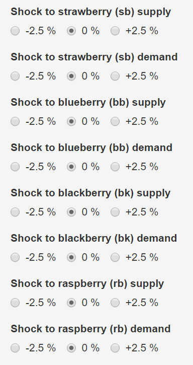
Notice from the table that the own-price demand elasticities are all in the elastic range. All the cross-price elasticities are positive indicating that consumers view the different types of berries as substitutes. Demonstration \(\PageIndex{2}\) presents the equilibrium model in matrix form. There are eight endogenous variables as shown in the column headings for the A matrix and in the solution vector. These consist of percentage changes in four quantities and four prices, corresponding to each of the four types of berries in the model. You can control exogenous demand or supply shocks using the radio buttons in the left panel of the demonstration. Take a moment to verify how the elasticities in Table \(\PageIndex{1}\) translate into matrix A in Demonstration \(\PageIndex{2}\).
Use Demonstration \(\PageIndex{2}\) to consider the effect of a positive supply shock to one of the markets. Make sure all demand shocks are set to zero, then add a positive supply shock to one and only one of the markets. This will increase revenue to producers in the market experiencing the positive supply shock. You can see this because the positive change in quantity is larger in magnitude than the negative change in price. The impact of the shock on producers in the remaining berry markets is negative. Demand decreases in each market not affected by the shock because the remaining berries are substitutes in demand.
Now consider the effect of a positive demand shock to one of the markets. Make sure all supply shocks are set to zero, then add a positive shock to one and only one of the markets. The impact is biggest on the market experiencing the demand shock but the spillover effects cause an increase in price and quantity in each of the related markets as well. Spend some time with the demonstration by considering other shocks to demand and or supply. if you want to test your knowledge, see if you can replicate this model in a spreadsheet or in R.
Demonstration \(\PageIndex{2}\). Interactive implementation of Sobekova’s (2012) model for retail fresh berry markets.
Matrix A
          Qsb Qbb Qbk Qrb   Psb   Pbb   Pbk   Prb
Supply sb   1   0   0   0 -0.29  0.00  0.00  0.00
Demand sb   1   0   0   0  1.26 -0.32 -0.52 -0.39
Supply bb   0   1   0   0  0.00 -0.09  0.00  0.00
Demand bb   0   1   0   0 -0.12  1.49 -0.24 -0.20
Supply bk   0   0   1   0  0.00  0.00 -0.09  0.00
Demand bk   0   0   1   0 -0.05 -0.06  1.88 -0.06
Supply rb   0   0   0   1  0.00  0.00  0.00 -0.12
Demand rb   0   0   0   1 -0.08 -0.10 -0.13  1.66
Vector b
          Pct. Shock
Supply sb          0
Demand sb          0
Supply bb          0
Demand bb          0
Supply bk          0
Demand bk          0
Supply rb          0
Demand rb          0
Solution Vector
    Pct. Change
Qsb           0
Qbb           0
Qbk           0
Qrb           0
Psb           0
Pbb           0
Pbk           0
Prb           0

