5.2: Neoclassical Consumer Theory

The basic idea behind consumer choice theory is very simple: The consumer seeks to obtain the best bundle of goods and services that he or she possibly can (Varian 1993). This is true of the neoclassical theory covered in this section as well as the extension to the theory to be described below. In deciding what is the best bundle of goods and services, economists generally assume that the consumer has preferences that can be represented by a utility function. The utility function assigns a number to a given bundle of goods and services. A bundle that the consumer likes more is assigned a higher number. A bundle that the consumer likes less is assigned a lower number. A utility function formalizes the idea that consumers have the ability to rank various bundles of goods and services in terms of their desirability.

Preferences represented by a utility function determine the “best” bundle of goods and services. However, think carefully about the fundamental idea that a consumer chooses the best bundle of goods and services that he or she possibly can. The “possibly can” part of the idea is very important. A consumer’s best bundle might include several multimillion-dollar homes: one at a ski resort in the Rockies or Alps, one on the north shore of Lake Superior (for summer months), and one in the Virgin Islands (for winter months when not on the ski slopes). Of course, the best bundle would also include a private jet to take the consumer wherever he or she fancied. Very few people could obtain this best bundle. This is because the dollars consumers have to spend is limited by their available income.

We could reformulate our fundamental idea in terms of economic jargon as follows: consumers maximize their utility subject to a budget or income constraint. The utility function determines what is best. The budget or income constraint determines the set of possible bundles that the consumer can obtain.

Budget Sets in the Neoclassical Model

The budget set contains all combinations of goods that the consumer can afford. In this course, simple budget sets that include only two goods will be used. Such a simplification may not work well in empirical applications using real-world data because each consumer probably has hundreds, if not thousands, of possible goods in their budget set (just think about the wide variety of goods available in any supermarket, department store, or online retailer). However, all models are simplifications, and in terms of understanding consumer choice behavior, a two-good world can get you a long way. With a simple two-good world you can develop an understanding of the essential logic of the consumer choice model. Simplifying the world to only two goods also allows the consumer’s choice space to be represented graphically (as in Demonstration 1 below).

Algebraically, the budget set is defined over the quantities of the two goods, \(Q_{1}\) and \(Q_{2}\) as all pairs:

\({Q_{1}, Q_{2}}: P_{1}Q_{1} + P_{2}Q_{2} \leq M,\)

where \(P_{1}\) and \(P_{2}\) are prices of goods 1 and and 2, respectively, and \(M\) is the consumer’s income. The budget set simply states that the amount spent on good 1 plus the amount spent on good 2 must be less than the consumer’s income.

The budget frontier consists of those bundles that completely exhaust the consumer’s income. In the expression for the budget set above, replace the inequality with an equal sign and you have those points that comprise the budget frontier. Because \(Q_{2}\) will be on the vertical axis this expression for \(Q_{2}\). This is the equation for the budget frontier:

\(Q_{2} = \dfrac{M}{P_{2}} - \dfrac{P_{1}}{P_{2}} Q_{1}.\)

An example budgets set is presented in Demonstration \(\PageIndex{1}\). Note that this is a line with a vertical intercept of \(\dfrac{M}{P_{2}}\) and a slope of \(-\dfrac{P_{1}}{P_{2}}\)

There is an easy way to graph the budget set in a two-good economy. The vertical intercept is where the consumer spends all of his or her income on good 2. You only need to ask how many units of good 2 the consumer could afford if the entire budget went to good 2. The answer is \(\dfrac{M}{P_{2}}\). The horizontal intercept can similarly be found be asking how many units of good 1 could be obtained if the consumer spend all his/her money on good 1, which is \(\dfrac{M}{P_{1}}\). Thus if you know \(M\), \(P_{1}\), and \(P_{2}\), you can, in a matter of seconds, graph the consumer’s budget frontier. Simply divide \(M\) by \(P_{2}\) to get your vertical intercept, divide \(M\) by \(P_{1}\) to get your horizontal intercept, and connect the dots. It is as easy as that! You now have your frontier. The budget set is comprised of the points on the frontier and the points south and west of the frontier.

Demonstration \(\PageIndex{1}\). The Budget Set

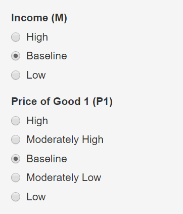
First, use Demonstration \(\PageIndex{1}\) to see what happens to the budget set when \(P_{1}\) and/or \(P_{2}\) changes. Start by increasing one of the prices, \(P_{1}\) or \(P_{2}\), but not both. The price increase changes the slope of the frontier because the intercept for the axis with the now higher-priced good moves towards the origin. The entire budget set becomes smaller. You will see a triangular area comprised of points that the consumer was able to afford before the price increase but can no longer afford afterwards. Now, go ahead and increase the other price as well. This further contracts the budget set. Finally, set the prices back to their initial values. Repeat the process for a price decrease and note what happens to the budget set. The takeaway here is that price changes affect both the size of the budget set and slope of the budget frontier.

Second, use Demonstration \(\PageIndex{1}\) to evaluate a change in income (\(M\)). Decrease the consumer’s income in the demonstration and notice that both the vertical and horizontal intercepts contract towards the origin. The budget frontier line makes a parallel shift to the southwest. The entire budget set becomes smaller. Repeat the process for an increase in income and note what happens to the budget set. The conclusion to be drawn is that a change in income affects the size of budget set but not the slope of the budget frontier.

Preferences in the Neoclassical Model

A budget set identifies what bundles are affordable to a consumer. The fundamental idea behind consumer theory is that a consumer will choose the best bundle from this set. Just what this “best” bundle is depends on the consumer’s preferences. To facilitate a discussion of preferences, it will be useful to introduce some preference relations that we can use to indicate how the consumer views different bundles. These relations are defined in Table \(\PageIndex{1}\).

Table 1. Preference Relations

Relation	Name	Example	Interpretation
\(\approx\)	Indifference	\(x \approx y\)	\(x\) is indifferent to \(y\)
\(\succeq\)	Weakly preferred	\(x \succeq y\)	\(x\) is at least as good as \(y\)
\(\succ\)	Strictly preferred	\(x \succ y \)	\(x\) is better than \(y\)

Representing Preferences Graphically

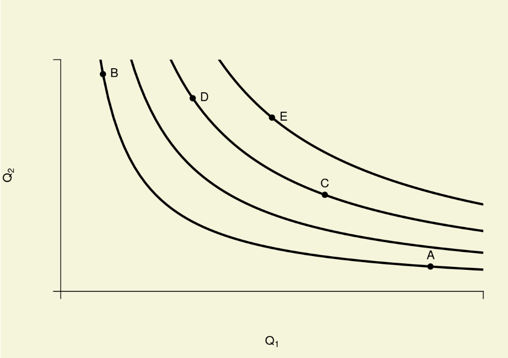
In introductory microeconomics, you probably learned about indifference curves (they might also have been called iso-utility curves). Figure \(\PageIndex{1}\) presents indifference curves that represent a consumer’s preferences. Each labeled point in Figure \(\PageIndex{1}\) represents a bundle of the two goods. The curves are called indifference curves because they represent bundles that the consumer likes equally well. Unless, you are instructed otherwise, you are to assume that points on indifference curves to the northeast are increasingly preferred. For instance, E is preferred to all labeled bundles on this diagram because it lies on the indifference curve that is furthest northeast. Based on Figure \(\PageIndex{1}\), it is possible to make the following statement about the five labeled bundles:

\(E \succ D \approx C \succ B \approx A.\)

Given the preference relations defined above, the following are also true, although less precise, statements of the preference ordering for the consumer with the preference map in Figure \(\PageIndex{1}\):

\(E \succeq D \succeq C \succeq B \succeq A,\)

and

\(E \succeq C \succeq D \succeq A \succeq B\)

Figure \(\PageIndex{1}\): Graphical representation of preferences.

Utility Functions

A preference map, such as that in Figure \(\PageIndex{1}\), is a two-dimensional representation of a utility function. The important thing about a utility function is that it assigns numbers that indicate the consumer’s strength of preference for a given bundle. If the consumer likes bundle C more than bundle A, then a utility function would assign a higher number to bundle C and a lower number to bundle A. If the consumer likes bundle B just as much as bundle A, then the utility function would assign the same number to both bundles A and B. There is an important concept here. This concept is that a utility function provides an ordinal (not cardinal) ranking of preferences. With an ordinal utility function, one does not particularly care about the utility number itself, only that higher numbers are assigned to bundles the consumer likes more, lower numbers to bundles the consumer likes less, and that the same number is assigned to bundles the consumer likes equally well.

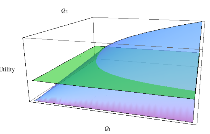
Figure \(\PageIndex{2}\) depicts a utility function. The function is in blue tones and shows the level of utility corresponding to different combinations of goods 1 and 2. The horizontal plane in the figure, depicted in green, intersects the utility function at a specified height. The intersection between the plane and function provides all combinations of goods 1 and 2 that provide the consumer with level of utility equal to the height of the plane. If you were to look at the utility function directly from above, you would see that the intersection of the plane with the function maps out an indifference curve. Thus, an indifference curve map, such as that shown in Figure \(\PageIndex{1}\), is actually a two dimensional representation of a three dimensional phenomenon. Each indifference curve depicts a given height on the utility function.

Figure \(\PageIndex{2}\): An indifference curve depcits the level of utility from a utility function.

Assumptions About Preferences

There are several assumptions that are commonly made about preferences. These assumptions simplify the consumer’s choice problem and also result in individual demand equations that conform to the law of demand.

Preferences are complete. If preferences are complete, it means that the consumer is able to rank bundles. This is not unreasonable assumption in most cases. If you were given a choice between two packages of almonds with one apple (bundle A) or one package of almonds with two apples (bundle B), you could probably indicate which bundle you most preferred or whether you were indifferent between the two.

Preferences are transitive. Transitive preferences simply mean that if \(C \succeq B\), and \(B \succeq A\), then it must be that \(C \succeq A\). Like completeness, transitivity is a fairly straightforward assumption. The transitivity assumption assures that indifference curves will never intersect one another.

That preferences are reflexive and continuous are additional basic assumptions about preferences which are important to formal mathematical treatment of consumer theory but are of less practical importance in a course like this. The important thing is that if preferences are complete, transitive, reflexive, and continuous; there is an ordering of preferences that can be represented by a utility function (Varian 1992). It is common to make two additional assumptions about preferences and these are of more practical importance in this course. The first is that preferences are convex and the second is that preferences are monotonic.

Preferences are convex. Convexity is a common assumption made about preferences. Given (1) the consumer likes bundle A exactly as much as bundle B \((A \approx B)\), and (2) bundle A is not the same bundle as bundle B (\(A \neq B\)), preferences are strictly convex if the consumer prefers an average bundle \(C = 0.5A + 0.5B\) to either bundle A or B by itself. Convexity implies that consumers like to have variety in their consumption. Another way to say this is that “means are preferred to extremes.”

In most cases, convexity is a reasonable assumption. It is actually hard to come up with cases where convexity might not hold. Suppose, for example, that a consumer likes cocktail olives and that the consumer also like chocolate ice cream. However, ice cream does not pair well with olives and so the the consumer does not like to have cocktail olives with his/her ice cream. In this case, you might argue that the consumer would prefer an extreme bundle (all cocktail olives or all ice cream) to a mean bundle (some cocktail olives and some ice cream) and his or her preferences would not be convex. This example is a bit stretched, however. It assumes that that the consumer would somehow be forced to eat cocktail olives and ice cream at the same time. Why could he or she not eat the ice cream now and save the olives for later? Over the course of the day, the consumer may want to have something sweet with lunch (ice cream) and something savory with supper (cocktail olives). Thus, even though he or she does not like cocktail olives and ice cream at the same time, preferences are still convex because the consumer likes a variety of sweet and savory foods over the course of a day.

Preferences are monotonic. The second additional assumption is that preferences are monotonic. Monotonicity simply means that the consumer prefers bundles with more goods to bundles with less. Given two bundles, bundles A and B, monotonicity means the consumer prefers B to A if:

1. B contains at least as much of each good as does A, and
2. B contains strictly more of at least one good than does A.

Is monotonicity a reasonable assumption? At first glance it would seem that it is not because there are some goods where too much of a good becomes a bad. For example, after eating two sandwiches, the consumer could be sick, literally, if forced to eat a third. That said, an argument can be made that monotonicity is a very reasonable assumption for models of the consumer. This is because consumers make market choices only in regions where their preferences are monotonic. For example, if a consumer is waiting in line to purchase a sandwich it is a pretty good assumption that an additional sandwich is something he or she wants and that preferences are monotonic at least with respect to one more sandwich. In short, consumers are only in the market when they want more of a good or when they have monotonic preferences for the good in question. The goal of the consumer model is to provide a reasonable approximation to what occurs in the real world. If, in the real world, consumers are only making choices in regions where monotonicity holds, then it is a reasonable to assume monotonicity for preferences used in the consumer model.

Choice in the Neoclassical Model

Having covered budget sets and preferences in some detail, let us now return to the basic idea of consumer theory: Consumers choose the best bundle of goods and services that they possibly can. The “best” part of the idea is given by preferences. The “possibly can” part of the idea is determined by budget sets. In the parlance of the model, the consumer’s problem is to achieve the highest indifference curve possible given the budget set.

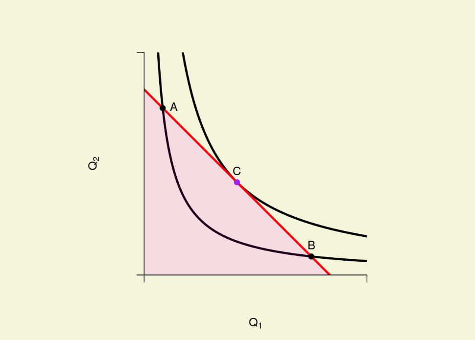
Figure \(\PageIndex{3}\) provides a graphical illustration of the consumer’s choice problem. Points A, B, and C are on the frontier of the budget set. At each of these points, the consumer is exhausting all of his/her income. Only point C, however, is optimal. Given convexity, point C is preferred to either A or B. As a result, our utility function places point C on a higher indifference curve. In fact, it is not possible to find a point within the consumer’s budget set that is preferred to point C. Thus, point C is the best bundle that the consumer can afford. At point C, the indifference curve is tangent to the budget frontier line.

Figure \(\PageIndex{3}\): Point C is the consumer’s optimal choice. If preferences are strictly monotonic and strictly convex, the optimal choice occurs where the indifference curve is tangent to the budget frontier line.

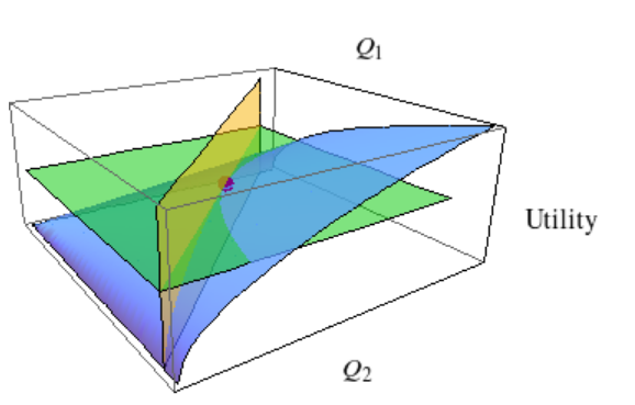
Again, Figure \(\PageIndex{3}\) is a two-dimensional representation of a three-dimensional phenomenon. Figure \(\PageIndex{4}\), depicts the utility function (blue-toned surface). The yellow-toned vertical plane intersecting the utility function is the budget constraint. The consumer cannot afford points and corresponding levels of utility that lie to the right of this vertical budget plane. The consumer’s goal is to reach the highest elevation on the utility function possible. In Figure \(\PageIndex{4}\), this highest level is shown by the purple point. The green-toned horizontal plane is set to the elevation of the affordable point that provides the greatest utility. If the model were to be viewed directly from above, this three-dimensional model would look very similar to the two-dimensional model in Figure \(\PageIndex{3}\). You would see an indifference curve that is created by the intersection of the green horizontal plane and the utility function. This indifference curve would just touch the vertical budget plane at the optimal point.

Figure \(\PageIndex{4}\): The neoclassical choice model in three dimensions.

Individual Demand Curves

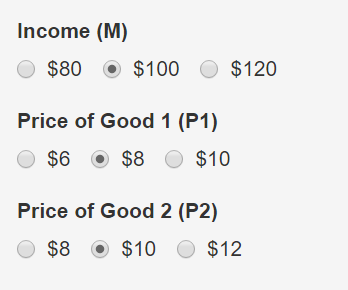
The theory of consumer choice, the idea that the consumers seek the highest point on their utility function given an affordability constraint, can be used to generate demand curves. This is illustrated in Demonstration \(\PageIndex{2}\) below. Notice that as \(P_{1}\) increases, the consumer’s budget set becomes smaller and his or her optimal choice changes to include a smaller amount of \(Q_{1}\). Conversely as \(P_{1}\) decreases, the consumer’s budget set becomes larger and his or her optimal choice includes a larger amount of \(Q_{1}\). The lower panel of the demonstration depicts a mapping of the optimal choices of \(Q_{1}\) corresponding to different levels of \(P_{1}\), holding \(P_{2}\) and \(M\) constant. The result is a nice, downward sloping, demand schedule. As you change the value of \(P_{1}\) in the demonstration, be sure to note the relationship between the choice model in the upper panel and the demand schedule in the lower panel.

Anything aside from own-price that effects the budget sets or the preference map shifts the individual demand curve. For example, in Demonstration \(\PageIndex{2}\), you can change the level of income. As you do this, notice that the budget set changes and the demand curve shifts. In general, any variable, aside from own-price, that affects the budget set or that effects the preference map will shift the individual’s demand schedule.

Demonstration \(\PageIndex{2}\). The Choice Model and the Consumer’s Individual Demand Schedule