31.31: The Aggregate Expenditure Model

Last updated
Save as PDF

Page ID: 51829

\( \newcommand{\vecs}[1]{\overset { \scriptstyle \rightharpoonup} {\mathbf{#1}} } \) \( \newcommand{\vecd}[1]{\overset{-\!-\!\rightharpoonup}{\vphantom{a}\smash {#1}}} \)\(\newcommand{\id}{\mathrm{id}}\) \( \newcommand{\Span}{\mathrm{span}}\) \( \newcommand{\kernel}{\mathrm{null}\,}\) \( \newcommand{\range}{\mathrm{range}\,}\) \( \newcommand{\RealPart}{\mathrm{Re}}\) \( \newcommand{\ImaginaryPart}{\mathrm{Im}}\) \( \newcommand{\Argument}{\mathrm{Arg}}\) \( \newcommand{\norm}[1]{\| #1 \|}\) \( \newcommand{\inner}[2]{\langle #1, #2 \rangle}\) \( \newcommand{\Span}{\mathrm{span}}\) \(\newcommand{\id}{\mathrm{id}}\) \( \newcommand{\Span}{\mathrm{span}}\) \( \newcommand{\kernel}{\mathrm{null}\,}\) \( \newcommand{\range}{\mathrm{range}\,}\) \( \newcommand{\RealPart}{\mathrm{Re}}\) \( \newcommand{\ImaginaryPart}{\mathrm{Im}}\) \( \newcommand{\Argument}{\mathrm{Arg}}\) \( \newcommand{\norm}[1]{\| #1 \|}\) \( \newcommand{\inner}[2]{\langle #1, #2 \rangle}\) \( \newcommand{\Span}{\mathrm{span}}\)\(\newcommand{\AA}{\unicode[.8,0]{x212B}}\)

The aggregate expenditure model relates the components of spending (consumption, investment, government purchases, and net exports) to the level of economic activity. In the short run, taking the price level as fixed, the level of spending predicted by the aggregate expenditure model determines the level of economic activity in an economy.

An insight from the circular flow is that real gross domestic product (real GDP) measures three things: the production of firms, the income earned by households, and total spending on firms’ output. The aggregate expenditure model focuses on the relationships between production (GDP) and planned spending:

\[GDP = planned\ spending= consumption + investment + government\ purchases + net\ exports.\]

Planned spending depends on the level of income/production in an economy, for the following reasons:

If households have higher income, they will increase their spending. (This is captured by the consumption function.)
Firms are likely to decide that higher levels of production—particularly if they are expected to persist—mean that they should build up their capital stock and should thus increase their investment.
Higher income means that domestic consumers are likely to spend more on imported goods. Since net exports equal exports minus imports, higher imports means lower net exports.

The negative net export link is not large enough to overcome the other positive links, so we conclude that when income increases, so also does planned expenditure. We illustrate this in Figure 31.2.22 "Planned Spending in the Aggregate Expenditure Model" where we suppose for simplicity that there is a linear relationship between spending and GDP. The equation of the line is as follows:

\[spending = autonomous\ spending + marginal\ propensity\ to\ spend \times real\ GDP.\]

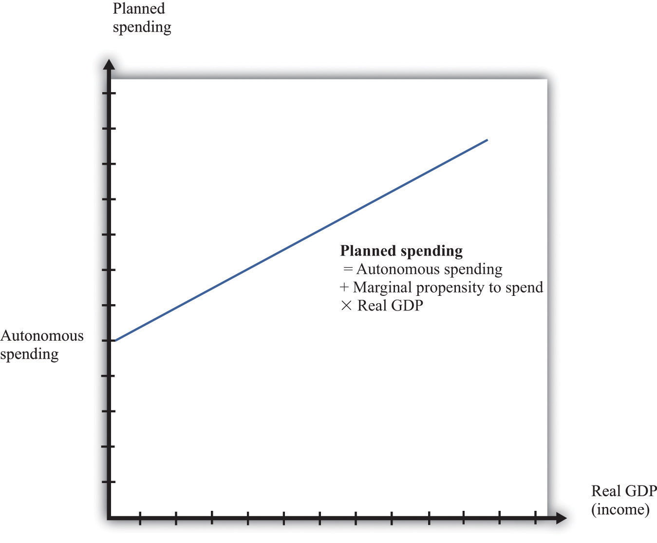
Figure \(\PageIndex{22}\): Planned Spending in the Aggregate Expenditure Model

The intercept in Figure 31.2.22 "Planned Spending in the Aggregate Expenditure Model" is called autonomous spending. It represents the amount of spending that there would be in an economy if income (GDP) were zero. We expect that this will be positive for two reasons: (1) if a household finds its income is zero, it will still want to consume something, so it will either draw on its existing wealth (past savings) or borrow against future income; and (2) the government would spend money even if GDP were zero.

The slope of the line in Figure 31.2.22 "Planned Spending in the Aggregate Expenditure Model" is given by the marginal propensity to spend. For the reasons that we have just explained, we expect that this is positive: increases in income lead to increased spending. However, we expect the marginal propensity to spend to be less than one.

The aggregate expenditure model is based on the two equations we have just discussed. We can solve the model either graphically or using algebra. The graphical approach relies on Figure 31.2.23. On the horizontal axis is the level of real GDP. On the vertical axis is the level of spending as well as the level of GDP. There are two lines shown. The first is the 45° line, which equates real GDP on the horizontal axis with real GDP on the vertical axis. The second line is the planned spending line. The intersection of the spending line with the 45° line gives the equilibrium level of output.

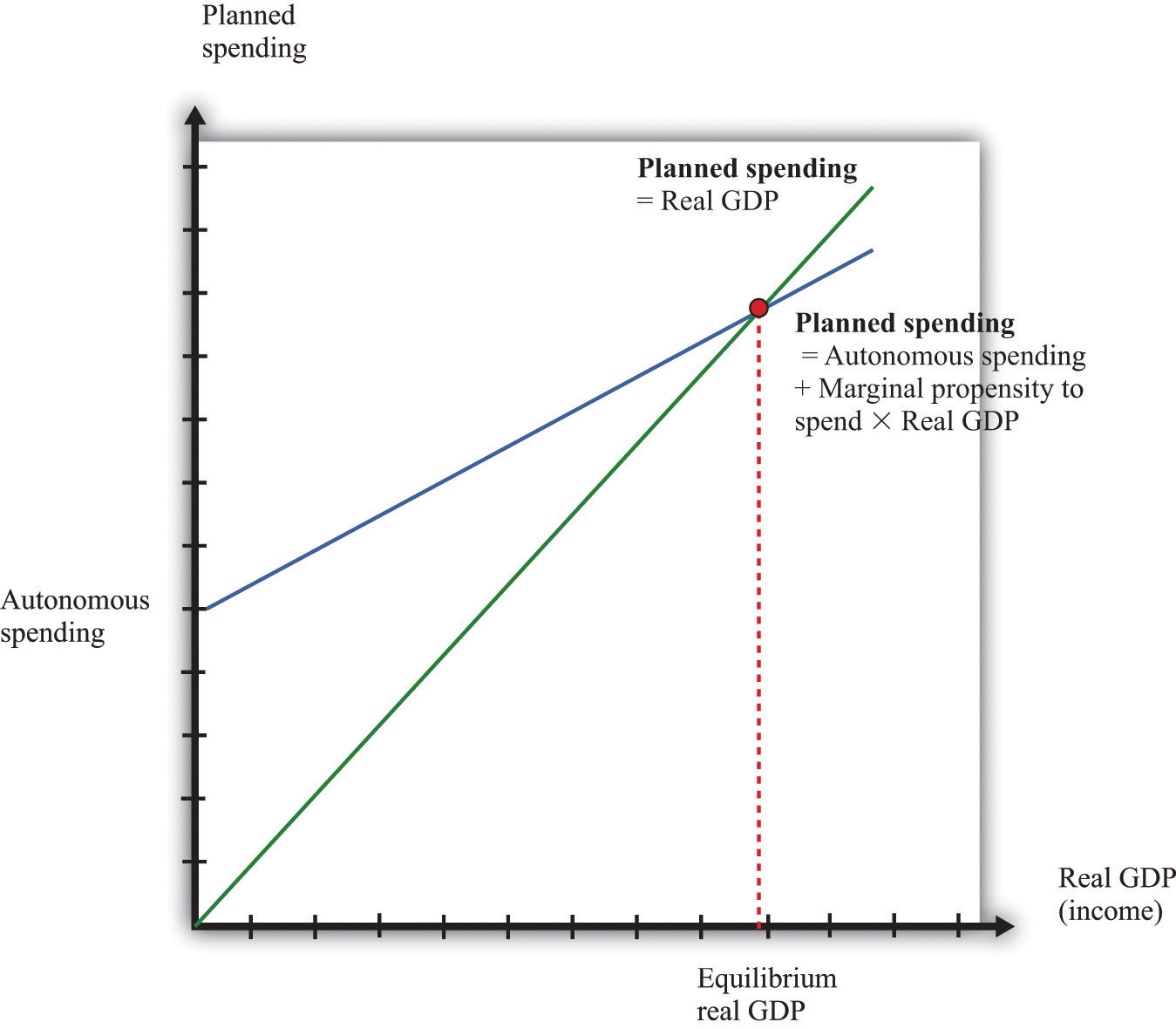
Figure \(\PageIndex{23}\)

More Formally

We can also solve the model algebraically. Let us use Y to denote the level of real GDP and E to denote planned expenditure. We represent the marginal propensity to spend by β. The two equations of the model are as follows:

\[Y = E\]

and

\[E=E_{0}+\beta \times Y\]

Here, E₀ is autonomous expenditure. We can solve the two equations to find the values of E and Y that are consistent with both equations. Substituting for E in the first equation, we find that

The equilibrium level of output is the product of two terms. The first term—\((1/(1 − \beta))\)—is called the multiplier. If, as seems reasonable, β lies between zero and one, the multiplier is greater than one. The second term is the autonomous level of spending.

Here is an example. Suppose that

C = 100 + 0.6Y,

I = 400,

G = 300,

and

NX = 200 − 0.1Y,

where C is consumption, I is investment, G is government purchases, and NX is net exports. First group the components of spending as follows:

\[C + I + G + NX = (100 + 400 + 300 + 200) + (0.6Y − 0.1Y)\]

Adding together the first group of terms, we find autonomous spending:

\[E_{0}= 100 + 400 + 300 + 200 = 1,000.\]

Adding the coefficients on the income terms, we find the marginal propensity to spend:

\[\beta = 0.6 − 0.1 = 0.5.\]

Using β = 0.5, we calculate the multiplier:

We then calculate real GDP:

\[Y = 2 \times 1,000 = 2,000.\]