3.2: More Practice and Understanding Solver

We know there are two approaches to solving optimization problems.

1. Analytical methods using algebra and calculus (conventional, paper and pencil, using the Lagrangean method): The idea is to transform the consumer’s constrained optimization problem into an unconstrained problem and then solve it using standard unconstrained calculus techniquesi.e., take derivatives, set equal to zero, and solve the system of equations.

2. Numerical methods using a computer (Excel’s Solver): Set up the problem in Excel, carefully organizing things into a goal, endogenous variables, exogenous variables, and constraint; then use Excel’s Solver. Use the Sensitivity Report in the Solver Results dialog box to get \(\lambda\mbox{*}\).

In this chapter, we apply both methods on a new problem.

Quasilinear Utility Practice Problem

A utility function that is composed of a nonlinear function of one good plus a linear function of the other good is called a quasilinear functional form. It is quasi, or sort of, linear because one good increases utility in a linear fashion and the other does not.

Below are a general example and a more specific example of quasilinear utility.

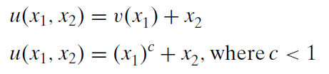
If \(c < 1\), then the quasilinear utility function says that utility increases at a decreasing rate as \(x_1\) increases, but utility increases at a constant rate as \(x_2\) increases.

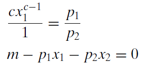
The optimization problem is to maximize this utility function subject to the usual budget constraint. It is written in equation form like this: \[\max\limits_{x_1,x_2,\lambda}x_1^c + x_2 \\ \textrm{s.t. } p_1x_1 + p_2x_2 = m\] We will solve the general version of this problem, with letters representing exogenous variables instead of numbers, using the Lagrangean method.

1. Rewrite the constraint so that it is equal to zero.

\(0 = m - p_1x_1 - p_2x_2\)

2. Form the Lagrangean function. \[\max\limits_{x_1,x_2,\lambda} {\large\textit{L}} = x_1^c + x_2 + \lambda(m -p_1x_1 - p_2x_2)\] Note that the Lagrangean function, L, has the quasilinear utility function plus the Lagrangean multiplier, \(\lambda\), times the rewritten constraint.

Unlike the concrete problem in the previous chapter, which used numerical values, this is a general problem with letters indicating exogenous variables. General problems, without numerical values for exogenous variables, are harder to solve because we have to keep track of many variables and make sure we understand which ones are endogenous versus exogenous. If the solution can be written as a function of the exogenous variables, however, it is often easy to see how an exogenous variable will affect the optimal solution.

3. Take partial derivatives with respect to \(x_1\), \(x_2\), and \(\lambda\).

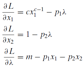
Remember that the partial derivative treats other variables as constants. Thus, the partial derivative of the quasilinear utility function with respect to \(x_1\) has no \(x_2\) variable in it.

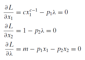
4. Set the derivatives equal to zero and solve for \(x_1\mbox{*}\), \(x_2\mbox{*}\), and \(\lambda\mbox{*}\).

We use the same solution method as before, moving the lambda terms to the right-hand side and then dividing the first equation by the second, which allows us to cancel the lambda terms.

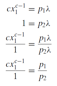
By canceling the lambda terms, we have reduced the three equation, three unknown system to two equations with two unknowns.

Remember that not all variables are the same. The endogenous variables, the unknowns, are \(x_1\) and \(x_2\). The other letters are exogenous variables.

From the first equation, we can solve for the optimal quantity of good 1 (see the appendix to the previous section if these steps are confusing).

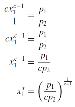
Notice that we used the rule that \((x^a)^b = x^{ab}\). Because we wanted to solve for \(x_1\), we raised both sides to the \(\frac{1}{c-1}\) power so that the \(c - 1\) exponent on \(x_1\) times \(\frac{1}{c-1}\) would equal 1.

Usually, when we have the MRS equal to the price ratio, we need to solve for one of the x variables in terms of the other and substitute it into the budget constraint. However, a property of the quasilinear utility function is that the MRS only depends on \(x_1\); thus by solving for \(x_1\), we get the reduced form solution. When solving a problem in general terms, the answer must be expressed as a function of exogenous variables alone (no endogenous variables) and this is called a reduced form.

To get \(x_2\), we simply substitute \(x_1\) into the budget constraint and solve for \(x_2\).

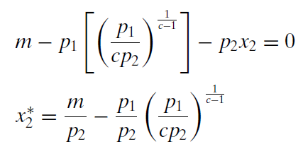
It is a bit messy, but it is the answer. We have an expression for the optimal amount of \(x_2\) that is a function of exogenous variables alone.

To get the optimal value of lambda, we can use the second first-order condition, which simply says that \(\lambda \mbox{*} = \frac{1}{p_2}\). If you use the first condition, substituting in the value for optimal \(x_1\), it will take a little work, but you will get the same result.

Practice with the MRS = \(\frac{p_1}{p_2}\) Logic

Economists stress marginal thinking. The idea is that, from any position, you can move and see how things change. If there is improvement, continue moving. The optimal solution is on a flat spot, where improvement is impossible.

When we move the lambda terms over to the right-hand side and divide the first equation by the second equation, we get a crucial statement of the fact that improvement is impossible and we are optimizing.

The familiar MRS equals the price ratio expression, along with the third first-order condition, which says that the consumer must be on the budget line (exhausting all income), is a mathematical way of describing marginal thinking.

The MRS condition tells us that if the MRS is not equal to the price ratio, there are two possibilities, depicted in Figure 3.7.

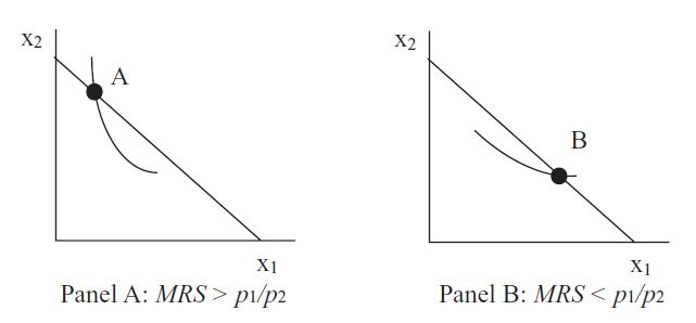Figure 3.7: MRS does not equal the price ratio.

In Panel A, the slope of the indifference curve at point A is greater than the slope of the budget line (in absolute value). This consumer should crawl down the budget line, reaching higher indifference curves, until the MRS equals the price ratio. At this point, the slope of the indifference curve will exactly equal the slope of the budget line and the consumer’s indifference curve will just touch the budget line. The consumer cannot possibly get to a higher indifference curve and stay on the budget constraint. This is the best possible solution.

In Panel B, the story is the same, but reversed. The slope of the indifference curve at point B is less than the slope of the budget line. This consumer should crawl up the budget line, reaching higher indifference curves, until the MRS equals the price ratio. At this point, the slope of the indifference curve will exactly equal the slope of the budget line and the consumer’s indifference curve will just touch the budget line.

Numerical Approach to Quasilinear Practice Problem

STEP Open the Excel workbook OptimalChoicePractice.xls, read the Intro sheet, and then go to the QuasilinearChoice sheet to see how the numerical approach can be used to solve this problem.

It is easy to see that the consumer cannot afford the bundle 5,20 given the prices and income on the sheet. If she buys five units of \(x_1\), what’s the maximum \(x_2\) she can buy?

STEP Enter this amount in cell B12. Does the chart and cell B21 confirm that you got it right?

If you entered 13 in B12, then the chart updates and shows that the consumer is now on the budget line. In addition, the constraint cell, B21, is now zero.

Without running Solver or doing any calculations at all, is she maximizing at 5,13?

The answer is that she is not. It’s hard to see on the chart whether the indifference curve is cutting the budget line, but the information below the chart shows that the MRS is not equal to the price ratio. That tells you that the indifference curve is, in fact, not tangent to the budget line so the consumer is not optimizing. Because the MRS is greater than the price ratio (in absolute value) we also know that the consumer should buy more \(x_1\) and less \(x_2\), moving down the budget line until the marginal condition is satisfied. Let’s find the optimal solution.

STEP Run Solver. Select the Sensitivity Report to get \(\lambda\mbox{*}\).

How does Excel’s answer compare to our analytical answer? Recall that we found:

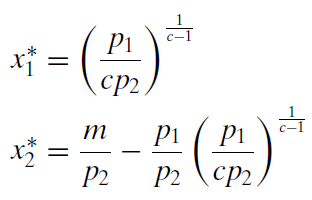
STEP Create formulas in Excel to compute these two solutions (using cells C11 and C12 would make sense). This requires some care with the parentheses. Here is the formula for good 1: =(p1_/(c_*p2_))(̂1/(c_-1)).

You should discover that Excel’s Solver is quite close to the exactly correct solution, 6.25, 12.75. We conclude that the two methods, analytical and numerical, substantially agree.

It is true, however, that Solver is ever so slightly off the computed analytical result. In general, there are two reasons for minuscule disagreement between the two methods.

1. Excel cannot display the algebraic result to an infinite number of decimal places. If the solution is a repeating decimal or irrational number, Excel cannot handle it. Even if the number can be expressed as a decimalfor example, one-half is 0.5precision error may occur during the computation of the final answer. This is not the source of the discrepancy in this case.

2. Excel’s Solver often misses the exactly correct answer by small amounts. Solver has a convergence criterion (that you can set via the Options button in the Solver Parameters dialog box) that determines when it stops hunting for a better answer. Figure 3.8 offers a graphical representation of Solver’s algorithm in a one-variable case.

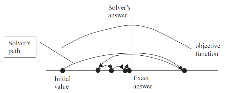Figure 3.8: Solver in action.

The stylized graph (which means it represents an idea without using actual data) in Figure 3.8 shows that Solver works by trying different values and seeing how much improvement occurs. The path of the choice variable (on the x axis) is determined by Solver’s internal optimization algorithm. By default, it uses Newton’s method (a steepest descent algorithm), but you can choose an alternative by clicking the Options button in the Solver dialog box.

When Solver takes a step that improves the value of the objective function by very little, determined by the convergence criterion (adjustable via the Options button), it stops searching and announces success. In Figure 3.8, Solver is missing the optimal solution by a little bit because, if we zoomed in, the objective function would be almost flat at the top. Solver cannot distinguish additional improvement.

When we say that the analytical method agrees with Solver, we do not mean that the two methods exactly agree, but simply that they correspond, in a practical sense. If Solver is off the exact answer in the 15th decimal place, that is agreement, for all practical purposes.

Furthermore, it is easy to conclude that Solver must give an exact answer because it displays so many decimal places. This is incorrect. Solver’s display is an example of false precision. It is not true that the many digits provide useful information. The exact answer is 6.25 and 12.75. What you are seeing is Solver noise. You must learn to interpret Solver’s results as inexact and not report all of the decimal places.

There is another way in which Solver can fail us and it is much more serious than incorrectly interpreting the results.

Solver Behaving Badly

STEP Start from \(x_1 = 1, x_2 = 20\) to see a demonstration that Solver is not perfect. After setting cells B11 and B12 to 1 and 20, respectively, run Solver. What happens?

A miserable result (an actual, technical term in the numerical methods literature) occurs when an algorithm reports that it cannot find the answer or displays an obviously erroneous solution. Figure 3.9 displays an example of a miserable result. Solver is clearly announcing that it cannot find an answer.

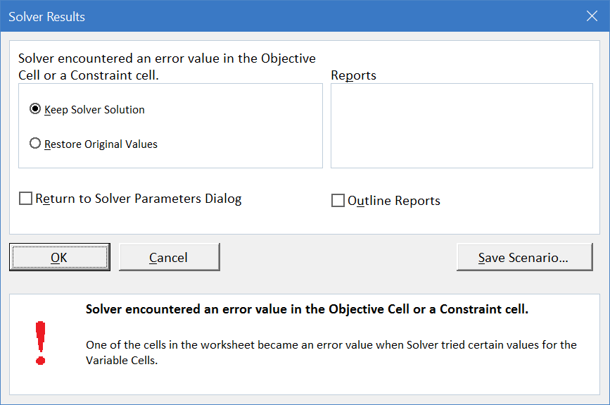Figure 3.9: A miserable result.

If you look carefully at the spreadsheet (click cancel or OK if needed to return to the sheet), you will see that Solver blew up when it tried a negative value for \(x_1\). The objective function cell, B7, is displaying the error #NUM! because Excel cannot take the square root of a negative number.

To be clear, when we start from 1,20, Excel tries to move left and crosses over the y axis into negative x territory. Since the utility function is \(x_1^{0.5}\), it tries to take the square root of a negative number, producing an error, and crashing the algorithm.

When Solver fails, there are three basic strategies to fix the problem:

1. Try different initial values (in the changing cells). If you know roughly where the solution lies, start near it. Always avoid starting from zero or a blank cell.
2. Add more structure to the problem. Include non-negativity constraints on the endogenous variables, if appropriate. In the case of consumer theory, if you know the buyer cannot buy negative amounts, add this information.
3. Completely reorganize the problem. Instead of directly optimizing, you can put Solver to work on equations that must be met. In this problem, you know that MRS \(= \frac{p_1}{p_2}\) is required. You could create a cell that is the difference between the MRS and the price ratio and have Solver find the values of the choice variable that force this cell to equal zero.

Let’s try the second strategy.

STEP Reset the initial values to 1 and 20, then launch Solver (click the Data tab and click Solver) and click the Add button (at the top of the stacked buttons on the right).

Solver responds by popping up the Add Constraint dialog box.

STEP Select both of the endogenous variables in the Cell Reference field, select \(>=\), and enter 0 in the Constraint field so that the dialog box looks like Figure 3.10. Click OK.

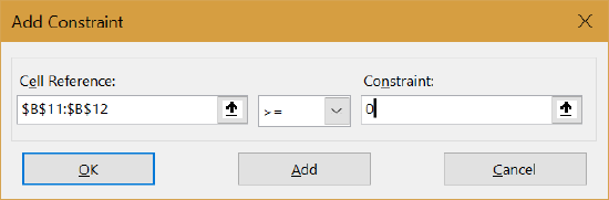Figure 3.10: A miserable result.

You are returned to the main Solver Parameters dialog box, but you have added the constraint that cells B11 and B12 must be non-negative.

You might notice that you could have have simply clicked the Make Unconstrained Variables Non-Negative option, but adding the constraint shows how to work with constraints.

STEP Once back at the main Solver Parameters dialog box, click Solve.

This time, Solver succeeds. Adding the non-negativity constraint prevented Solver from trying negative \(x_1\) values and producing an error.

Perfect Complements Practice Problem

Recall that L-shaped indifference curves represent perfect complements, which are reflected via the following mathematical function:

\[u(x_1,x_2) = min{ax_1,bx_2}\] Suppose \(a = b = 1\) and the budget line is \(50 = 2x_1 + 10x_2\).

First, We want to solve this problem analytically.

The Lagrangean method cannot be applied because the function is not differentiable at the corner of the L. The Lagrangean method, however, is not the only analytical method available. Figure 3.11 shows that when a = b = 1, the optimal solution must lie on a ray from the origin with slope +1.

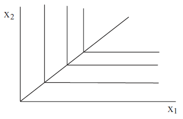Figure 3.11: The optimal solution line with perfect complements.

The optimal solution has to be on the corner of the L-shaped indifference curves because a non-corner point (on either the vertical or horizontal part of the indifference curve) implies the consumer is spending money on more of one of the goods without getting any additional satisfaction. Thus, we know that the optimal solution must lie on the line \(x_2 = x_1\).

We can combine this optimal solution equation with the budget constraint to find the optimal solution. The two equation, two unknown system can be solved easily by substitution.

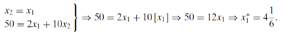
Of course, we know \(x_2 = x_1\) so optimal \(x_2\) is also \(4 \frac{1}{6}\). Can Excel do this problem and do we get the same answer? Let’s find out.

STEP Proceed to the PerfectComplements sheet to see how we set up the spreadsheet in Excel. Click on cell B7 to see the utility function.

STEP Run Solver and get a Sensitivity Report. Solver can be used to generate a value for the Lagrangean multiplier (via the Sensitivity Report) even though we could not use the Lagrangean method in our analytical work.

As with the previous problem (with quasilinear utility), we find that Solver and the analytical approach substantially agree. The answer is a repeating decimal, so Excel cannot get the exact answer, \(4 \frac{1}{6}\), but it is really close.

Previously, we saw that Solver could crash and give a miserable result. Now, let’s learn that Solver can really misbehave.

STEP Starting from \(x_1 = 1, x_2 = 1\), run Solver. What happens?

You are seeing an example of a disastrous result which occurs when an algorithm reports that it has found the answer, but it is wrong. There is no obvious error and the user may well accept the answer as true.

Solver reports a successful outcome, but the answer it gives is 1,1 and we know the right answer is \(4 \frac{1}{6}\) for both goods.

Disastrous results include an element of interpretation. In this case, we might notice that 1,1 is way inside the budget constraint and, therefore, the algorithm has failed. A truly disastrous result occurs when there is no way to independently test or verify the algorithm’s wrong answer.

Miserable and disastrous results are well defined, technical terms in the mathematical literature on numerical methods. Disastrous results are much more dangerous than miserable results. The latter are frustrating because the computer cannot provide an answer, but disastrous results lead the user to believe an answer that is actually wrong. In the world of numerical optimization, they are a fact of life. Numerical methods are not perfect. You should never completely trust any optimization algorithm.

Understanding SolverBe Skeptical

This chapter enabled practice solving the consumer’s constrained optimization problem with two different utility functions, a quasilinear function and perfect complements. In both cases, we found that Excel’s Solver agreed, practically speaking, with the analytical method.

The ability to solve optimization problems with two independent methods means we can be really sure we have found an optimal solution when they give the same answers.

In addition, we explored how Solver actually works. It evaluates the objective function for different values of the choice variables. It continues searching for a better solution until it cannot improve much (an amount determined by the convergence criterion).

Solver can fail by reporting that it cannot find a solution (called a miserable result) oreven worseby reporting an incorrect answer with no obvious error (which is a disastrous result).

It is easy to believe that a result displayed by a computer is guaranteed to be correct. Do not be careless and trustingnumerical methods can and do fail, sometimes spectacularly.

This point deserves careful repetition. You run Solver and it happily announces that a solution has been found and offers up a 15 or 16 digit number for your inspection. The problem, however, is that the solution is way off. Not in the millionth or even tenth decimal place, but completely, totally wrong. How this might happen takes us too far afield into the land of numerical optimization, but suffice it to say that you should always ask yourself if the answer makes common sense.

Solver really is a powerful way to solve optimization problems, but it is not perfect. You need to always remember this. After running Solver, format the results with an eye toward ease of understanding and think about the result itself. Do not mindlessly accept a Solver result. Stay alert even if Solver claims to have hit pay dirtit may be a disastrous result!

More explanation of Solver is available in the SolverInstructions.doc file in the SolverCompStaticsWizard folder.

Exercises

1. In the quasilinear example in this chapter, use the first equation in the first-order conditions to find \(\lambda\mbox{*}\). Show your work.
2. Use analytical methods to find the optimal solution for the same perfect complements problem as presented in this chapter, except that \(a = 4\) and \(b = 1\). Show your work.
3. Draw a graph (using Word’s Drawing Tools) of the optimal solution for the previous question.
4. Use Excel’s Solver to confirm that you have the correct answer. Take a picture of the cells that contain your goal, endogenous variables, and exogenous variables.

References

As economics became more mathematical, a new course was born, Math Econ. The course needed books and R. G. D. Allen’s Mathematical Analysis for Economists (first published in 1938) became a classic textbook. As E. Schneider, a reviewer, said, “This book fills a long-felt want. At last we possess a book which presents the mathematical apparatus necessary to a serious study of economics in a form suited to the needs of the economist.” See The Economic Journal, Vol. 48, No. 191 (September, 1938), p. 515. The epigraph is from page 2 of Mathematical Analysis for Economists, as Allen discusses how and why mathematics can be applied to the study of economics.