5.1: Introduction to the Endowment Model

Last updated
Save as PDF

Page ID: 58456

$ \newcommand{\vecs}[1]{\overset { \scriptstyle \rightharpoonup} {\mathbf{#1}} } $ $ \newcommand{\vecd}[1]{\overset{-\!-\!\rightharpoonup}{\vphantom{a}\smash {#1}}} $$\newcommand{\id}{\mathrm{id}}$ $ \newcommand{\Span}{\mathrm{span}}$ $ \newcommand{\kernel}{\mathrm{null}\,}$ $ \newcommand{\range}{\mathrm{range}\,}$ $ \newcommand{\RealPart}{\mathrm{Re}}$ $ \newcommand{\ImaginaryPart}{\mathrm{Im}}$ $ \newcommand{\Argument}{\mathrm{Arg}}$ $ \newcommand{\norm}[1]{\| #1 \|}$ $ \newcommand{\inner}[2]{\langle #1, #2 \rangle}$ $ \newcommand{\Span}{\mathrm{span}}$ $\newcommand{\id}{\mathrm{id}}$ $ \newcommand{\Span}{\mathrm{span}}$ $ \newcommand{\kernel}{\mathrm{null}\,}$ $ \newcommand{\range}{\mathrm{range}\,}$ $ \newcommand{\RealPart}{\mathrm{Re}}$ $ \newcommand{\ImaginaryPart}{\mathrm{Im}}$ $ \newcommand{\Argument}{\mathrm{Arg}}$ $ \newcommand{\norm}[1]{\| #1 \|}$ $ \newcommand{\inner}[2]{\langle #1, #2 \rangle}$ $ \newcommand{\Span}{\mathrm{span}}$$\newcommand{\AA}{\unicode[.8,0]{x212B}}$

This chapter introduces a wrinkle to the standard consumer theory model that greatly enhances its applicability. Instead of treating income as a given cash amount, we model the consumer as having a given initial endowment of goods that can be traded for other goods. This transforms the consumer into a combined consumer and seller.

Although the power of this approach may not be immediately obvious, we will see that a wide variety of examples such as saving/borrowing, charitable giving, and much more can be handled with this modification.

The Budget Constraint in an Endowment Model

Instead of the usual income (m) variable, an Endowment Model is characterized by a budget constraint that equates expenditures and revenues from sales out of the initial endowment. \[p_1x_1 + p_2x_2 = p_1 \omega _1 + p_2 \omega _2\] The term on the right-hand side says that the consumer has a given amount of each good, $\omega _1$ and $\omega _2$ (this is Greek letter omega so we have omega-one and omega-two). Because the initial amounts of each good are given, $\omega _1$ and $\omega _2$ are exogenous variables.

The starting amount of each good, the coordinate pair $\omega _1$, $\omega _2$, is called the initial endowment. If we multiply the initial amount of each good by the price of that good, as done in the right-hand side of the budget constraint equation, we get a dollar-valued amount that represents the total income that can be raised by selling the entire endowment.

Thus, the budget constraint says that spending (on the left-hand side) must equal the value of the consumer’s assets (on the right-hand side).

The classic example to illustrate someone operating with an endowment model constraint is a farmer who goes to market with his crop. He sells his produce and, with the revenue obtained by selling, buys other goods. The core idea is that the farmer is a buyer and a seller.

Perhaps a more modern example is eBay. People sell all kinds of products and turn around and buy different products. It is a massive online garage-sale community. Once again, the core idea is that eBayers sell and buy.

In an Endowment Model, what the agent can buy depends on how much revenue is generated by sales. High prices for goods to be sold are a good thing from the agent’s point of view because they generate a lot of revenue with which to buy other goods.

Because Endowment Models transform the consumer into a combined buying-selling agent, we can get different results than we saw in the Standard Model. One critical difference is that price increases lead to decreases in quantity demanded (assuming the good is normal), as usual, but as price keeps rising, we can cross the zero barrier and get negative quantity demanded! We will see that the agent switches from being a buyer to being a seller. This is a key idea.

Let’s put these abstract ideas into concrete examples so we can understand what is going on with the Endowment Model.

STEP Open the Excel workbook EndowmentIntro.xls, read the Intro sheet, then go to the MovingAround sheet. Follow the instructions on the sheet to learn how we can create a budget line from a single point.

Just like the Standard Model, the agent faces a consumption possibilities frontier, also known as the budget line, that shows the feasible combinations. Bundles beyond the line are unattainable.

STEP Proceed to the Properties sheet.

Notice how we can use the value of the endowment to measure the agent’s "income." Starting with 35,10 and $p_1 = 2, p_2 = 3$, the value of the endowment is $100 ($70 from $x_1$ and $30 from $x_2$). The most $x_2$ the agent can have is $33 \frac{1}{3}$, the y intercept and the maximum $x_1$, the x intercept, is 50.

The highlighted circle in the graph (reproduced as Figure 5.1) represents the initial endowment. From the initial allocation of 35,10, the agent can move northwest, selling $x_1$ and buying $x_2$. Or, the agent can decide to acquire even more $x_1$ by selling $x_2$ and buying $x_1$, which means traveling in a southeasterly direction. The slope of the constraint is the usual price ratio.

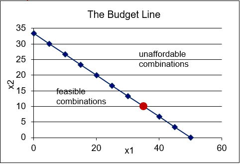
Fig1BC copy.png — Figure 5.1: Endowment Model budget constraint.

Source: *EndowmentIntro.xls!Properties*

What will the consumer do in terms of buying and selling? In other words, where will the agent end up on the budget line? We do not know because we do not have any information on this agent’s preferences. Before we tackle that problem, however, we need to see how the budget constraint changes when an exogenous variable is shocked.

STEP Proceed to the Changes sheet. Change $p_1$ (in K9) from 2 to 5.

This is different than before. Instead of the budget constraint pivoting about the y intercept (as in the standard, cash-income model), your screen should look like Figure 5.2. The budget constraint has pivoted or rotated as it did before, but the rotation is around the initial endowment. This is a critical difference.

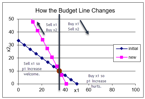
Figure 5.2: Endowment Model $p_1$ increase.

Source: *EndowmentIntro.xls!Changes*

The way the budget constraint has changed reveals important information. The price increase has improved the agent’s consumption possibilities if she is planning on traveling northwest on the constraint. This makes sense because she would be a seller of good 1 and, with the higher price, she would have more money with which to buy good 2.

On the other hand, if she is a buyer, then we get the usual result that the budget line has rotated in and reduced the consumption possibilities.

STEP Click the button and change $p_1$ (in K9) from 2 to 1.

Notice how the budget line has swiveled around the endowment again, but this time the agent is worse off if she is a seller and better off if she is a buyer.

STEP Click the button and change $p_2$ (in K10) from 3 to 6. The result is exactly the same as when you changed $p_1$ (in K9) from 2 to 1.

This reveals a lesson: All that matters in the Endowment Model are relative prices, $\frac{p_1}{p_2}$. So $p_1=1, p_2=3$ is the same as $p_1=2, p_2=6$ and $p_1=10, p_2=30$ and any $p_1$ and $p_2$ whose $p_1/p_2$ ratio is $\frac{1}{3}$.

Finally, we consider shifts in the budget constraint. We cannot shift m (cash income) like we did in the Standard Model, but we can shock the initial endowment quantities of goods and this acts like a shift in income.

STEP Click the button and change $\omega _1$ (in K13) from 35 to 50.

The chart now looks like the usual increase in income in the Standard Model.

STEP Click the button and change $\omega _2$ (in K14) from 10 to 2.

This generates a downward shift in the budget constraint. So price changes cause rotations (or pivots or swivels) and endowment shocks produce shifts.

The budget constraint in an Endowment Model plays the same role as the budget constraint in the Standard Model. It describes the agent’s consumption possibilities. Unlike the Standard Model, however, where price changes caused rotation around the x or y intercept, price shocks in the Endowment Model lead to swiveling around the initial endowment. It makes sense that the initial endowment is going to remain the same as prices change because the agent is neither buying nor selling at the initial endowment so the price does not matter at that point.

To get shifts in the budget constraint, we will have to change either $\omega _1$ or $\omega _2$. This changes the initial endowment point and allows the agent to buy and sell from the new endowment point, creating a new budget line.

Now that you understand the budget constraint, we are ready to solve the agent’s constrained utility maximization problem with the Endowment Model.

The Initial Solution

The utility side of the Endowment Model is the same as the Standard Model. The agent’s preferences are shown by indifference curves that are represented mathematically by a utility function.

The agent seeks to maximize utility given the budget constraint. As usual, we can solve this problem numerically and analytically.

STEP Proceed to the OptimalChoice sheet. Figure 5.3 shows what this sheet looks like when you first open it.

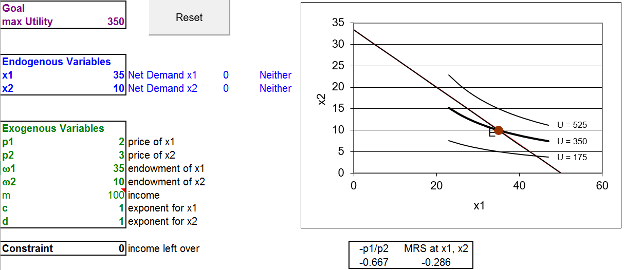
Figure 5.3: The initial view of the optimization problem.

Source: *EndowmentIntro.xls!OptimalChoice*

Notice how the organization is the same as the Standard Model. There is a goal, endogenous variables (in blue) and exogenous variables (in green). The agent seeks to maximize utility, represented by a Cobb-Douglas functional form, by choosing the amounts of $x_1$ and $x_2$ to consume, subject to the budget constraint.

The graph is also similar, with the addition of point E, representing the initial endowment. There are three representative indifference curves (there are an infinity of such curves, one through every point in the quadrant).

Although much is familiar, Figure 5.3 and your computer screen do have some notable innovations. Cells B18 and B19 have been added to the list of exogenous variables. They represent the given initial endowment. Cell B20 has a formula that computes m, which is not bolded to indicate that it is derived from other exogenous variables.

In addition, cells C11:E12 are new. Let’s find out what they tell us.

STEP Click on D11 to see its formula, = x1_ - w1_.

The underscore (_) is used to distinguish the names, x1 and w1, from the cell addresses, X1 and W1. Lowercase w is the closest English character to $\omega$.

More substantively, the formula computes net demand, how much the consumer wants to buy or sell. It takes gross demand, the optimal amount of the good the agent wishes to end up with, that is, the values of $x_1$ and $x_2$ and subtracts the initial endowment amounts. There is a gross and net demand for each good.

On opening, the net demand for $x_1$ is zero because B11 is set at 35, which is equal to the agent’s initial endowment of good 1. Suppose the agent decided to buy three units of good 1.

STEP Change B11 to 38.

Net demand for good 1 is now plus three. That makes sense because the consumer started with 35 units of good 1, but wants to have 38, so three more must be purchased.

Of course, the combination 38,10 is unattainable. The consumer must sell some $x_2$ in order to be able to buy three units of $x_1$. How much needs to be sold? Two units.

STEP Change B12 to 8.

The agent is back on the budget line and net demand for good 2 is negative. Cell E12 reports that the agent is a seller of good 2. Clicking on cell E12 reveals an IF formula that displays Buyer or Seller depending on whether net demand is positive or negative.

Compare the MRS on your screen to the MRS at the initial position from Figure 5.3. Was buying three units of good 1 with the proceeds from the sale of two units of good 2 a smart move?

No. The MRS at 38,8 is farther away from the price ratio than the MRS at 35,10. The graph reveals that we moved to a lower indifference curve when we moved to 38,8.

We need to head the other way. The agent needs to travel up the budget line, to the northwest, selling good 1 and buying good 2. How much should be sold and bought?

STEP Run Solver to find the initial solution.

Utility is maximized when gross demands are 25 and $16 \frac{2}{3}$ of goods 1 and 2, respectively. Net demands are $- 10$ and $6 \frac{2}{3}$. This means the agent sells 10 units of good 1 and uses the $20 in revenue to buy $6 \frac{2}{3}$ units of good 2.

This is the same solution as in the Standard Model with $m = \$100.$ That makes sense, since the value of the initial endowment is $100.

We can confirm this result with analytical methods. We follow the recipe for the Lagrangean method of solving constrained optimization problems.

We will work on a general form of this problem, leaving all exogenous variables as letters to get a reduced form expression that we can evaluate for any combination of exogenous values. We rewrite the constraint to that it is equal to zero and form the Lagrangean.

The third step is to take derivatives with respect to each choice variable and in the final step we set the three derivatives equal to zero to get the first-order conditions, which we need to solve for $x_1 \mbox{*}, x_2 \mbox{*}$, and $\lambda \mbox{*}$.

Math2FOC copy.png

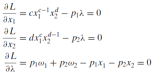
Our solution strategy involves moving the lambda terms to the right-hand side and dividing the first equation by the second to cancel lambda (and giving the familiar MRS = $\frac{p_1}{p_2}$ condition). This equation can then be solved for optimal $x_2$ as a function of optimal $x_1$.

Math3x2 copy.png

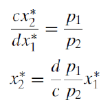
Although it looks like it, this is not the answer for $x_2$ because it has $x_1$ in it. The reduced form solution must be a function of exogenous variables alone. Substitute this expression for $x_2$ into the third first-order condition (the budget constraint) and solve for optimal $x_1$.

Math4x1Star copy.png

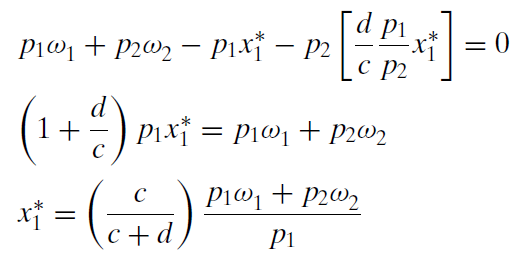
This expression can be evaluated for any combination of exogenous variable values. For example, if we use the parameter values in the OptimalChoice sheet, we can compute that optimal $x_1$ = 25. This agrees perfectly with the numerical approach.

Furthermore, this expression shows the quantity demanded at a given $p_1$, ceteris paribus, so it can be used to display a demand curve for $x_1$. There is, of course, a similar expression for good 2.

In the Standard Model, the reduced form solution was $x_1 \mbox{*} = (\frac{c}{c+d})\frac{m}{p_1}$. The Endowment Model’s solution is the same, except instead of m in the numerator, we have $p_1\omega _1 + p_2\omega _2$. This makes sense since the value of the initial endowment is $p_1\omega _1 + p_2\omega _2$.

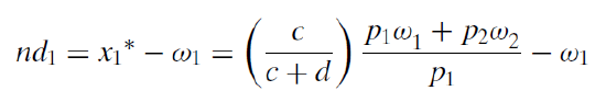
With an Endowment Model, we can subtract the initial amount of good 1 to obtain a net demand curve.

Math5ND1 copy.png

Comparative Statics with the Endowment Model

We can do comparative statics analyses analytically or numerically. The reduced form expression can be used to explore the rate of change of optimal $x_1$ with respect to any exogenous variable. For example, we can take the derivative with respect to $p_1$.

This is more complicated than usual because $p_1$ appears in two places. We could use the Product Rule, but it is easier to do some reorganizing and simplify things before we take the derivative.

First, we move $p_1$ from the denominator. This will enable us to use our usual derivative rule. \[x_1 \mbox{*} = (\frac{c}{c+d})\frac{p_1 \omega_1+p_2 \omega_2}{p_1}=(\frac{c}{c+d})(p_1 \omega_1+p_2 \omega_2)p_1^{-1}\] But we can also multiply $p_1$ through to cancel the $p_1$ in the $p_1 \omega_1$ term. \[x_1 \mbox{*} = (\frac{c}{c+d})(p_1 \omega_1+p_2 \omega_2)p_1^{-1} = (\frac{c}{c+d})(\omega_1+p_1^{-1}p_2 \omega_2)\] Then we can expand to leave $p_1$ isolated in a single term so that the derivative with respect to $p_1$ is straightforward. \[x_1 \mbox{*} = (\frac{c}{c+d})(\omega_1+p_1^{-1}p_2 \omega_2) = (\frac{c}{c+d})\omega_1+(\frac{c}{c+d})p_1^{-1}p_2 \omega_2\] Now, when we take the derivative with respect to $p_1$, we apply our usual derivative rule and bring the exponent down and subtract one from the second term. The first term has a derivative with respect to $p_1$ of zero since it does not contain $p_1$. \[\frac{dx_1 \mbox{*}}{dp_1} = (-1)(\frac{c}{c+d})p_1^{-2}p_2 \omega_2\] We can evaluate this expression at the initial values of the exogenous variables to get an instantaneous rate of change in optimal $x_1$ as $p_1$ changes. Plugging in $c = d = 1, p_1=2, p_2=3$, and $\omega _2=10$ gives $- 3.75$. This means that an infinitesimally small increase in $p_1$ would decrease $x_1$ by 3.75-fold.

But what does that number tell us? Is it a lot in the sense of a big response to a price shock? The slope provides no answer to this question. We need percentage changeselasticityto answer this question.

We can multiply the slope by the initial ratio of $\frac{p_1}{x_1 \mbox{*}}$ to compute the $p_1$ elasticity of $x_1 \mbox{*}$.

\[\frac{dx_1 \mbox{*}}{dp_1}\frac{p_1}{x_1 \mbox{*}} = ((-1)(\frac{c}{c+d})p_1^{-2}p_2 \omega_2)(\frac{p_1}{x_1 \mbox{*}})\] We evaluate this expression at $p_1 = 2$ (and the initial values of the other exogenous variables). \[\frac{dx_1 \mbox{*}}{dp_1}\frac{p_1}{x_1 \mbox{*}} = ((-1)(\frac{c}{c+d})p_1^{-2}p_2 \omega_2)(\frac{p_1}{x_1 \mbox{*}})=-3.75(\frac{2}{25}) \approx -0.3\] The elasticity does tell us that the quantity demanded of $x_1$ is quite price insensitive at the initial solution. An elasticity less than one (in absolute value) is said to be inelastic and the closer to zero, the lower the responsiveness.

Unlike the Standard Model, where a Cobb-Douglas utility function gives a unit price elasticity, we get a non-unitary elasticity here because a change in $p_1$ appears in the denominator and numerator in the reduced form. In the numerator, the change in price is affecting the value of the agent’s endowment whereas in the Standard Model, income is fixed.

We can also use numerical methods to explore the comparative statics properties of an own price change.

STEP Use the Comparative Statics Wizard to decrease $p_1$ by 0.1 (10 cents) for 15 shocks (from 2 to 0.5). Be sure to keep track of net demands and the buyer/seller position in the endogenous variables by using the ctrl key to select non-contiguous cells, as depicted in Figure 5.4. You want to track cells B11:B12 and D11:E12.

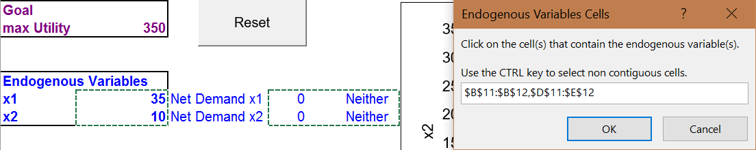Figure 5.4: Selecting endogenous variables with CSWiz.

The CSP1 sheet shows what your results should look like. There are several notable outcomes.

When the price fell from 90 cents to 80 cents, the agent switched from selling $x_1$ and buying $x_2$ to buying $x_1$ and selling $x_2$. The price of $x_1$ got so low that even though the agent starts with a lot of $x_1$ (compared to $x_2$), it is better to buy more $x_1$. The budget line gets flatter as $p_1$ falls, making buying $x_1$ a better choice than selling it.

Notice the behavior of maximum utility (column B) as price falls. The agent was a seller at first so falling prices hurt. Below 90 cents, however, the agent is a buyer of $x_1$ and falling $p_1$ increases utility.

The CSP1 sheet also shows slope and elasticity computations. From $p_1$ $2/unit to $1.90, the slope (yellow background) and elasticity (orange background) measures are close, but different than at $p_1=2$ (using the derivative). This is due to the fact that optimal $x_1$ is non-linear in $p_1$. In other words, $x_1 \mbox{*} = f(p_1)$ is not a line, but a curve (as clearly shown in the chart below the data).

The Endowment Model Extends the Standard Model

The Endowment Model is the Standard Model of the Theory of Consumer Behavior with an initial endowment of goods instead of cash income. This transforms the consumer into the dual-role of seller and buyer of goods. The driving force in the agent’s decision making remains utility maximization. Many of the ideas behind the Standard Model (such as equating the MRS and price ratio) carry over to the Endowment Model. Of course, the framework for presenting and understanding the model, comparative statics analysis, remains the same.

It may seem that replacing income with an initial endowment is a minor twist, but we will see that the Endowment Model enables analysis of a wide range of choice problems.

Exercises

Perform a comparative statics analysis of c, the exponent on $x_1$, using the Comparative Statics Wizard. Use increments in c of 0.1. State the effect of changing c on $x_1 \mbox{*}$. Describe your procedure and take screen shots of your results as needed.
Use your comparative statics results to find the c elasticity of $x_1 \mbox{*}$ from 1 to 1.1. Show your work.
Use the reduced form expression in this chapter to find the c elasticity of $x_1 \mbox{*}$. Show your work.
Compare your answers from questions 2 and 3. Explain why they are the same or differ.

References

The epigraph is from page 188 of David M. Kreps A Course in Microeconomic Theory (1990). If you are interested in graduate study in economics, this book is worth browsing. In the preface, Kreps says (p. xv),

The primary target for this book is a first-year graduate student who is looking for an introduction to microeconomic theory that goes beyond the traditional models of the consumer, the firm, and the market.

Kreps allows that it could be used for undergraduate majors taking an "advanced theory" course or "mathematically sophisticated students," but he warns that, "The book presumes, however, that the reader has survived the standard intermediate microeconomics course."

The Endowment Model is taking us close to the next level of microeconomic theory. Google "graduate micro theory" for more advanced micro books.

To learn more about Masters and PhD programs in economics, search for "graduate economics rankings" and be sure to visit the American Economics Association’s website at www.aeaweb.org/resources/students/grad-prep.