5.4: An Economic Analysis of Insurance

Why do people buy insurance?

If you are an economist, the answer is easy: because it makes them better off. According to economists, people solve an optimization problem and it turns out that those who buy insurance end up with greater satisfaction, on a higher indifference curve, than if they did not buy insurance.

We will use an Endowment Model to explain how and why insurance is an optimal choice. We will see yet another application of how to solve a constrained utility maximization problem and perform comparative statics analyses.

But the really deep lesson is that the Theory of Consumer Behavior is amazingly flexible and can answer questions from a wide range of problems. In this chapter, we have explored why people save and borrow, give to charity, and, now, buy insurance.

First, we will set up the problem with the usual constraint, indifference curves, and initial optimal solution (with MRS equal to the slope condition). The presence of risk, a probability that an event occurs, throws a curveball into the analysis, but we will convert things into our usual framework.

Second, we will do comparative statics. For example, we derive a demand curve for insurance. We can explore the effects of a higher premium, the price of insurance, on the quantity of insurance demanded. We are on the lookout for the premium elasticity of insurance.

An Endowment Model of Insurance

There are three parts to every optimization problem. In this case, we have the following:

1. Goal: maximize satisfaction (as represented by the utility function).
2. Endogenous variables: consumption in two states of nature, good and bad; by choosing the amount of insurance, we control two choice variables at once.
3. Exogenous variables: initial assets, potential loss, probability of loss, insurance premium, and preferences over the states of nature.

As usual, we start with the constraint, then turn to preferences, and finally use the constraint and utility function to find the initial solution.

STEP Open the Excel workbook Insurance.xls and read the Intro sheet, then go to the Constraint sheet.

The idea is that you have an asset, say your car or house, which may suffer a given amount of damage from an accident, called the PotentialLoss, with a known probability, \(\pi\) (the Greek letter, pi) that the damage occurs. Initially, the PotentialLoss is $10,000, which is only a fraction of the value of the house.

You can buy K dollars of insurance, this is the InsuredAmount, by paying a price (called a premium) of \(\gamma\) (the Greek letter, gamma) per $100 of insurance coverage. On opening, you are not buying any insurance.

If you buy insurance, then if the accident occurs, you get reimbursed for the loss. You can buy insurance in $100 increments, up to the PotentialLoss, in which case you would be fully insured. The trade-off is that you have to pay for insurance up front, before you know if the accident will happen or not.

After you decide how much insurance to buy, there are two possible outcomes, known as states of nature: the bad and good outcomes.

STEP Click on cell B18 to see the formula for your consumption in the bad outcome.

The ConsumptionBad outcome means the accident actually occurred, leaving your consumption as \(InitialAssets - PotentialLoss + K - \gamma K\). You subtract the loss that occurred and the amount you paid for insurance (\(\gamma K\)), but you add the amount K that the insurance company pays you because you suffered the accident. You could be fully covered, but you do not have to be. You decide how much insurance to buy.

Your consumption in the good state of nature is simply \(InitialAssets - \gamma K\). You do not suffer the accident, but you still have to pay for the insurance.

STEP Click on cell B19 to see the formula for the good outcome.

Cells B23:B25 display in which state of nature you end up. Cell B23 has the formula "=RAND()." This draws a number from a uniform distribution on the interval [0,1].

STEP Hit the F9 key on your keyboard repeatedly to understand Excel’s RAND() function works.

Each time you hit the F9 key, Excel draws a random number from 0 to 1 in cell B23. The number drawn is never smaller than zero or bigger than one.

Cell B24 converts the random draw in the cell above it into a zero or a onezero means the accident did not happen (good outcome) and one means it did (bad outcome). It uses an IF statement to display a "1" (the accident happened) when the random draw is less than 0.01 (the value of \(\pi\) in cell B8).

It is hard to see that anything is really happening in cell B24 because the probability of the accident occurring is so small.

STEP Change \(\pi\) to 50%, then hit F9 a few times. You should be able to see cell B24 flip from 0 to 1 and back again as the random draw is less than 0.5 and greater than 0.5.

Notice that the FinalAssets variable, cell B25, depends on whether or not the accident occurred.

Next, let’s buy some insurance to see what that does to the spreadsheet.

STEP Click the button and set cell B13 to $1000. This will cost you $10.

Notice the values for the good and bad states of nature. You have altered both. If the accident occurs, your consumption is $25,990, which is $990 better than the $25,000 for the bad outcome when you did not buy insurance. Of course, the good outcome is $10 lower (at $34,990) in the good outcome because you have to pay for the insurance even when the accident does not occur.

STEP Click the 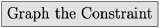button. Click OK to the "4" points default option and read each text box as it appears. At the end, the budget line is displayed (see Figure 5.16).

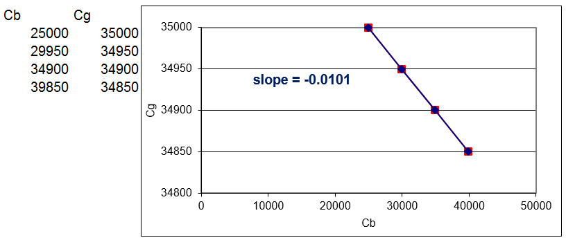
Figure 5.16: The budget line.

Source: Insurance.xls!Constraint

From the initial endowment (\(C_b, C_g\) without insurance), you can move down the budget line by buying insurance. You lower your consumption in the good state of nature (\(C_g\) is on the y axis), but raise it in the bad state of nature (\(C_b\) is on the x axis).

The terms of trade (the slope of the budget line) are determined by gamma (the insurance premium). The slope of the budget line is \(-\frac{\gamma}{1-\gamma}\), which with \(\gamma = 0.01\) is \(\frac{-1}{99}=0.01\) (the "01" keeps repeating forever). The graph rounds the slope to five decimal places.

Changes in initial assets or potential loss shift the budget constraint. We are interested, however, in deriving a demand curve for insurance so we will shock the insurance premium (the price of insurance). This will pivot or rotate the budget line.

STEP Change the insurance premium to $1.20 per $100 of insurance coverage.

You see the familiar swinging in (clockwise rotation) from a \(p_1\) increase. A buyer of insurance would be disappointed in this shock because her consumption possibilities are diminished.

Now that we understand the constraint, we turn to the agent’s tastes. We model utility as preferences over the two states of nature. The fact that there is risk involved in which state of nature occurs complicates things.

Instead of having utility simply depend on the amount of consumption in the good and bad outcomes, we include the agent’s expectations about the chances of each outcome occurring. Fortunately, our usual Cobb-Douglas functional form can incorporate this new information.

We use the exponents in the Cobb-Douglas functional form to represent the agent’s beliefs about the probability of the accident occurring. There are two simplifying assumptions. The first is that the agent accurately gauges the probability of loss, which means we can use \(\pi\) as the exponent in the utility function. The second assumption uses the fact that there are only two mutually exclusive outcomes so the bad outcome occurs with probability \(\pi\) and the good outcome has likelihood \(1-\pi\). The possibility of a partial loss is assumed away.

The utility function is then \[U=C_b^\pi C_g^{1-\pi}\] The idea behind the utility function is simple: The higher the probability of loss, the more the agent will care about the bad outcome. In terms of the indifference map, the higher \(\pi\), the steeper the indifference curves. This means the agent cares more about consumption in the bad state of nature as risk rises.

Unlike the Standard Model where the exponents in the Cobb-Douglas utility function can be used to represent changes in preferences, changes in the exponents do not indicate a change in preferences for the utility function with risk. To get a change in preferences, we need an entirely different utility function.

It is beyond the scope of this book, but there is a great deal of research on choosing with random outcomes. The field of behavioral economics was born with the discovery of paradoxes, violations of transitivity and other inconsistencies, when people made choices involving randomness. Our Cobb-Douglas utility function can be written as an expected utility function by simply taking the natural log: \[ln U=\pi C_b + (1-\pi)C_g\] This function reflects risk averse preferences. It is a starting point for modeling attitudes and feelings toward risk and randomness.

STEP Proceed to the Preferences sheet to see an implementation of the Cobb-Douglas utility function.

The sheet tries to give a new way of understanding how constrained utility maximization works. It shows consumption in the bad and good states of nature, $25,000 and $35,000, respectively, without insurance. This is the initial endowment point.

With \(\pi = 1\%\), we can compute the level of utility for the initial endowment combination of consumption in the bad and good states of nature. This is shown in cells D13 and E13. We can also compute the MRS at the initial endowment, displayed in cells G13 and H13.

The Dead and Live utility and MRS are the same because we are at the initial endowment. The Dead cells are numbers. They will not change when we change the cells in column B. The Live cells contain formulas. They will update when you change the values of \(C_b, C+g\), and \(\pi\).

STEP Ponder and answer the question in cell A6. Click on the when you are ready. Do the same for B10.

The Live utility and MRS cells change when you change cells B13 and B14. As you moved down from the initial endowment, utility rose and the MRS fell. It got closer to the slope which means we are closer to the optimal solution.

We are ready to find the initial optimal solution.

STEP Proceed to the OptimalChoice sheet.

The OptimalChoice sheet reproduces the Constraint sheet, but it adds the indifference map to the chart and displays the slope of the budget line and the MRS at the bottom of the chart. It also displays the utility in cell B20 from the chosen consumption in the two states of nature.

It is really hard to see what is happening with the indifference curve at the initial endowment and the slope of the budget line.

STEP Zoom indouble-click the y axis and make the minimum bound 34800 and the maximum bound 35200.

You can now see clearly that when MRS \(>\) slope of the budget line, the budget line cuts the indifference curve. By moving down the budget line, you can reach higher levels of satisfaction.

STEP Enter 5000 in cell B13 to see where the agent stands when buying $5000 of insurance.

The chart shows movement down the budget line to a higher level of utility. We are closer to the optimal solution, but not there yet because MRS is not equal to the slope of the budget line.

STEP Run Solver to find the optimal solution.

The Solver dialog box is notable for the fact that there are no constraints. The way we implemented the problem in Excel enabled us to directly maximize the utility cell by choosing a single variable, the amount of insurance purchased. We can still use, however, the canonical Theory of Consumer Behavior graph to show the result.

At the optimal solution, the consumer decides to buy $10,000 of insurance.

In the bad state, if the accident occurs, the agent is fully covered, so is consumption $35,000? No, because the agent has to pay $100 for the insurance, so consumption would be $34,900 in the bad state.

In the good state, where there is no accident, consumption is also $34,900. This is surprising. Insurance has removed the effect of risk. Consumption is the same in both states. This is an extreme example of diversification.

Diversification is a strategy to lower risk by spreading your wealth over different states of nature. By moving $100 from the good state of nature (buying insurance), the agent has a guaranteed level of utility regardless of whether the accident happens. Without insurance, the expected return is $34,900 since 99% x $35,000 + 1% x $25,000 = $34,900. But the agent has to put up with the risk of every 1 in 100 times getting $25,000. By diversifying, the expected return is the same, $34,900, with absolutely no risk.

Such a perfect resultthe complete elimination of riskrelies on the fact that the two states of nature are perfectly correlated. In the real world, when states of nature are not perfectly correlated (such as the stock market), diversification can lower risk while maintaining the same expected return, but it cannot completely eliminate it.

We know that people buy insurance because it increases satisfaction. This application models choosing the amount of insurance that maximizes utility subject to the budget constraint. Next, we use the model to derive a demand curve for insurance.

Comparative Statics

The procedure is straightforward: we vary the insurance premium (the price of insurance), \(\gamma\), ceteris paribus, and track the optimal amount of insurance purchased (K) to derive a demand curve for insurance.

We use numerical methods and leave the analytical work for the exercises.

STEP In the OptimalChoice sheet, change \(\gamma\) to $1.30 per $100 of insurance. What happens?

The budget line (displayed in red on your screen) gets steeper. The agent needs to re-optimize.

STEP Run Solver to find the new optimal solution.

If you did not zoom in on the y axis as instructed earlier, it is hard to see on the chart, but the cells below the chart confirm that the MRS equals the slope of the budget line when the agent buys $1847 of insurance.

We can conclude that demand for insurance is downward sloping when the premium rises from $1.00 to $1.30 since the amount of insurance purchased fell from $10,000 to $1847. That is extremely responsive.

STEP Compute the price elasticity of demand. Proceed to the CSgamma sheet to check your answer. Notice that Excel tries to help when you enter the formula by formatting the result as dollars. This is incorrect. Elasticity is unitless.

The CSgamma sheet shows that the CSWiz add-in was used to explore the effect of the insurance premium on the amount of insurance purchased. Gamma was incremented by 0.1 (10 cents) with 10 shocks. Optimal \(K, \gamma K, C_b,\) and \(C_g\) were tracked as \(\gamma\) changed. The sheet includes a chart of \(K \mbox{*} = f(\gamma)\), the demand curve for insurance.

Notice the curious behavior of the model as \(\gamma\) rises: at $1.40, optimal K becomes negative. This is an Endowment Model. When premium prices get high enough, the agent switches from buying insurance to selling insurance!

If this option is not allowed, you can impose the constraint in Excel that K be greater than or equal to zero. Then, with high premiums, the consumer is at a corner solution and buys no insurance.

Modeling Insurance via the Endowment Model

Insurance is another application of an Endowment Model in the Theory of Consumer Behavior. The usual ideas were applied: the budget constraint, preferences, and MRS equals slope of budget line at the optimal solution. In addition, the usual recipe of the economic approach, finding the initial optimum and then comparative statics, was followed.

But this application does have its own twists and novelties. We used a Cobb-Douglas functional form to model satisfaction where the exponents reflect the probabilities of the states of nature. We also used Excel’s Solver without a budget constraint because of the way we implemented the problem in Excel. To be clear, this problem can be solved via the Lagrangean method (see the first exercise question) and we could have implemented a "max U subject to a constraint" model in Excel. We would get, of course, the same answer.

Exercises

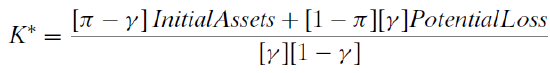
1. Use analytical methods to derive a general reduced form solution for \(K \mbox{*}\). Show your work.

   Although you can use the Lagrangean method, it is easier to maximize the utility directly, substituting in the values for each state of nature. \[\max\limits_{K}U=C_b^\pi C_g^{1-\pi }\] The key is that consumption in the good and bad states of nature depends on K: \[C_b = InitialAssets - PotentialLoss + K - \gamma K\] \[C_g = InitialAssets - \gamma K\] We can simply substitute these equations into the utility function and maximize this: \[\max\limits_{K}U=[InitialAssets - PotentialLoss + K - \gamma K]^\pi [InitialAssets - \gamma K]^{1-\pi}\]

2. Compare the analytical versus numerical approaches by evaluating your answer to question 1 at the initial parameter values in the OptimalChoice sheet. (Click the button if needed.) Do you find that \(K \mbox{*} = \$10,000\)?
3. Use your reduced form for K* to find the probability of loss elasticity of insurance demand at \(\pi\) = 1%. Show your work. If you cannot find the reduced form, use
4. Use the Comparative Statics Wizard to find the probability of loss elasticity of insurance demand from \(\pi = 1\%\) to 1.1%. Take a picture of your results, including the elasticity calculation.
5. Compare your answers in question 3 and 4. Do these elasticities differ? Why or why not?

References

The epigraph is from the first page of Foundations of Insurance Economics by Georges Dionne and Scott E. Harrington, editors, published in 1990. Insurance economics as an organized subfield is quite young, but rapidly growing. It focuses economics, probability, and computer science on applied problems in the world of risk and insurance.

In their wildly popular Freakonomics: A Rogue Economist Explores the Hidden Side of Everything (2005), Steven D. Levitt and Stephen J. Dubner include this example from the world of insurance markets:

In the late 1990s, the price of term life insurance fell dramatically. This posed something of a mystery, for the decline had no obvious cause. Other types of insurance, including health and automobile and homeowners’ coverage, were certainly not falling in price. Nor had there been any radical changes among insurance companies, insurance brokers, or the people who buy term life insurance. So what happened? The Internet happened. In the spring of 1996, Quotesmith.com became the first of several websites that enabled a customer to compare, within seconds, the price of term life insurance sold by dozens of different companies. (p. 66)

The freakonomics.com website has podcasts and other resources.