12.1: Initial Solution

With a total cost function, \(TC(q)\), and its associated average and marginal cost curves, we are ready to solve the the firm’s output profit maximization problem. The firm chooses the amount of output that maximizes profit, defined as total revenue minus total cost. This is the second of three optimization problems that make up the Theory of the Firm.

All firms face this profit maximization problem, but this chapter works with a perfectly competitive (PC) firm in the short run (SR). There are, of course, many other market structures and types of firms, but perfect competition is the first step from which more sophisticated scenarios arise.

The firm’s market structure tells us the environment in which it operates. Its market structure determines the firm’s revenue function. A PC firm is the simplest case because it takes price as given. Thus, revenues are simply price times quantity and the revenue function is linear.

Remember that we are not trying to describe the actual operation of a business. In fact, a truly perfectly competitive firm does not exist in the real world. The concept is an abstraction that enables derivation of the supply curve. This is our goal.

Remember also that the short run is defined by the fact that at least one input (usually K) is fixed. In the long run, the firm is free to choose how much to use of every factor. K is fixed not because it is immovable (like a pizza oven or a building), but because the firm has contracted to rent a certain amount. It cannot increase or decrease the amount of K in the short run.

Profit maximization and its graphs may be familiar from introductory economics. This experience will help you, but do not be complacent. Keep your eye on how the economic way of thinking is being applied in this case and make connections with other optimization problems we have explored.

Perfectly Competitive Market Structure

A perfectly competitive firm sells a product provided by countless other firms selling that homogeneous (which means identical) product to perfectly informed consumers. Because the product is homogeneous, there are no quality differences or other reasons for consumers to care about who they buy from. Because consumers are perfectly informed, they know the price of every seller.

Thus, the PC firm’s market structure is one of intense price competition. Every firm sells the product at the exact same price because if anyone tried to sell at even a tiny bit higher than the market price, no one would buy from them.

The shorthand term for this environment is price taking. The PC firm must take the price and cannot choose its priceprice is exogenous to the firm.

In addition to price taking, the market structure of the PC firm is characterized by an assumption about the movement of other firms into and out of the industry: free entry and exit. Firms can enter or leave the market, selling the same good as everyone else, at any time.

These two ideas, price taking and free entry, distinguish the PC firm from its polar opposite, monopoly. A monopolist chooses price and has a barrier to entry. Between these two extremes are many other market structures in which real-world firms actually exist.

The PC firm’s market structure means that an individual PC firm does not worry about what other firms are doing. Each firm simply chooses its own output to maximize profit and does not watch the other firms to gain a strategic advantage. In this sense, there is no rivalry in perfect competition.

Setting Up the Problem

As usual, we organize the optimization problem into three parts:

1. Goal: maximize profits (\(\pi\), Greek letter pi), which equal total revenues (TR) minus total costs (TC).
2. Endogenous variable: output (q).
3. Exogenous variables: price of the product (P), input prices (the wage rate (w) and the rental rate of capital (r)), and technology (parameters in the production function).

Unlike the consumer’s utility maximization and the firm’s input cost minimization problems, this profit maximization problem is unconstrained. The firm does not have a restriction, like a budget constraint or isoquant, that limits its choice of output to a particular range. It can choose any non-negative level of output.

This greatly simplifies the optimization problem. For the analytical method, it means we do not need the Lagrangean method. All we need to do is take a single derivative and set it equal to zero.

Finding the Initial Solution

Suppose the cost function is: \[TC(q) = aq^3 + b q^2 + c q + d\] Then we can form the PC firm’s profit function and optimization problem like this: \[\max\limits_{q} \pi=TR-TC\] \[\max\limits_{q} \pi=Pq-(aq^3 + b q^2 + c q + d)\] As usual, we have two ways to solve this optimization problem: numerically and analytically.

STEP Open the Excel workbook OutputProfitMaxPCSR.xls and look over the Intro sheet.

The Intro sheet is not meant to be immediately understood. It offers highlights of material that will be explained and prints as one landscaped page. It provides a compact summary of the optimal solution of the output profit maximization problem for a perfectly competitive firm in the short run.

STEP Proceed to the OptimalChoice sheet to find the initial solution.

The sheet is organized into the components of an optimization problem, with goal, endogenous, and exogenous variable cells.

Initially, the firm is producing nine units of output and making $11.74 of profit. Is this the highest profit it can possibly make?

No. The sheet reveals the information needed to give this answer. By comparing marginal revenue (MR) and marginal cost (MC), we immediately know that the firm would make a mistake (we would say it is inefficient) if it produced just nine units.

The MC of the ninth unit is $3.52 as shown in cell B22, but what about MR? Perhaps you remember from introductory economics that \(P=MR\) for perfectly competitive firms? We can see that the additional revenue produced by the last unit, $7 (the price), is greater than the additional cost, $3.52 (cell B22). Thus, the firm should produce more. How much exactly should the firm produce?

STEP Run Solver to find out.

Look carefully at B22. At the optimal solution, \(q \mbox{*} \approx 13.09\), MC = $7 per unit. \(P = MC\), a special case of \(MR=MC\) for a PC firm, is the equimarginal condition in this problem, analogous to \(MRS = \frac{p_1}{p_2}\) and \(TRS = \frac{w}{r}\). When the equimarginal condition is met, the firm is guaranteed to be maximizing profits.

To find the optimal solution via the analytical method, we take the derivative of the profit function with respect to q, set it equal to zero, and solve for \(q \mbox{*}\). Our cubic cost function introduces the complication that the solution has two roots so we have to use the quadratic formula.

STEP Click the 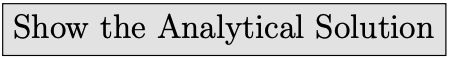button to see how to solve this problem with calculus.

Cell AC17’s formula has the root that maximizes profits (the other root minimizes profitsmore on this in the next section). As usual, Solver and calculus agree (not exactly, but they give effectively the same answer).

Representing the Optimal Solution with Graphs

Since this is an unconstrained optimization problem (unlike utility maximization and input cost minimization), the graphical display of the optimal solution is different.

The firm’s output profit maximization problem is usually represented by a graph that depicts the family of cost curves along with marginal and average revenue. Figure 12.1 and the Intro sheet shows this canonical graph for a perfectly competitive firm (signaled by the fact that firm demand is horizontal, so marginal revenue equals demand).

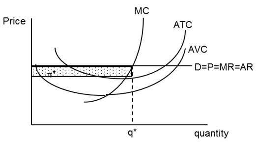
Figure 12.1: The canonical output profit maximization graph.

Source: OutputProfitMaxPCSR.xls!Intro.

Figure 12.1 is the usual display of the optimal solution, but it is actually part of a much larger graphical display.

STEP Proceed to the Graphs sheet to see how Figure 12.1 fits into the bigger picture, also shown in Figure 12.2. Zoom out to see all four graphs.

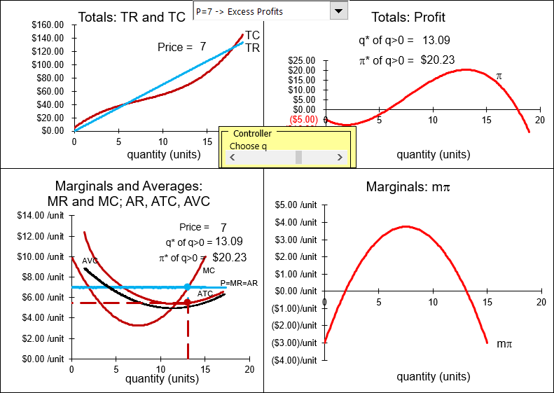
Figure 12.2: Four graphs of output profit maximization.

Source: OutputProfitMaxPCSR.xls!Graphs.

Each of the four graphs in Figure 12.2 and on your screen can be used to show the firm’s optimization problem and its solution. We will walk through each one.

1. The top left graph plots total revenue and total cost. TR is linear because the firm’s market structure is perfect competition, hence, it is a price taker. The cubic total function produces the shape of TC. The firm wants to choose q to maximize the difference between revenues and costs.
2. The top right graph shows the profit function, which is \(TR - TC\). The firm wants to choose q so that it is at the highest point on the profit hill.
3. The bottom right graph displays marginal profit, which can be expressed as the derivative of the profit function with respect to q. The firm can find the maximum profit by choosing q so that marginal profit is zero. This is the first-order condition from the analytical solution.
4. Finally, the bottom left graph is the usual display. The firm chooses q where MR (which equals P given that the firm is a price taker) equals MC. Profits can be calculated as the area of the rectangle \((AR - ATC)q\).

To be clear, all four graphs in Figure 12.2 show the same optimal q and maximum profits, but the graph that is most often used is the bottom left. It highlights the comparison of MR and MC and the family of cost curves provides information about the firm’s cost structure. We can also find profits as the area of the rectangle (with blue top and dashed line bottom).

STEP Move the output with the slider control (in the middle of the four charts) to the left and right of \(q \mbox{*}\) to see how the profit rectangle changes.

Only when q is such that \(MR = MC\) do you get the maximum area of the profit rectangle. Moving left from optimal q, you can make the rectangle taller, but you must make it shorter to do this and you end up with less area. You can make the rectangle longer by moving right from optimal q, but ATC rises and the rectangle gets thinner, so once again the area falls.

The intersection of MR and MC immediately reveals the optimal q. Profits at any q are also easily seen as the area of a rectangle, length times width, with units in dollars. Because the y axis is a rate, $/unit, and the x axis is in units of the product, multiplying the two leaves dollars. In other words, say the product is milk in gallons. Then price, average total, and average variable cost are all in $/gallon. Suppose that at a price of $2/gallon, MR = MC at an output of 7,000 gallons and ATC = $1.50/gallon at this output. Clearly, profits are ($2/gallon - $1.50/gallon) x 7,000 gallons, which equals $3,500.

We can compute profits from the profit rectangle at any level of output. The height of the rectangle is always average revenue (which equals price) minus average total cost. This vertical distance is average profit. When multiplied by the level of output, we get profits, in dollars, at that level of output.

The bottom left graph has another advantage over the other graphs. It can be used to explain a curious and puzzling feature of a firm’s short run profit maximization problem. The story revolves around a firm with negative profits and what it should do in this situation.

The Shutdown Rule

The firm has an option when maximum profits are negative: it can simply shut down, close its doors, hire no workers, and produce nothing. The Shutdown Rule says the the firm will maximize profits by producing nothing (\(q \mbox{*} = 0\)) when \(P < AVC\).

The key to whether the firm shuts down or continues production in the face of negative profits lies in its fixed costs. If the firm can do better by shutting down and paying its fixed costs instead of producing and choosing the level of output where \(MR = MC\), then it should produce nothing.

Continuing production in the face of negative profits versus shutting down are actually the last two of four possible profit positions for the firm.

1. Excess Profits: \(\pi \mbox{*} > 0 \text{ and } P > ATC\)
2. Normal Profits: \(\pi \mbox{*} = 0 \text{ and } P = ATC\)
3. Negative Profits, Continuing Production: \(\pi \mbox{*} < 0 \text{ and } P \geq AVC\)
4. Shutdown: \(\pi \mbox{*} < 0 \text{ and } P < AVC\)

Case 1, excess profits, occurs whenever maximum profits are positive. The example we have been working on is this case. With P = 7, we know that \(q \mbox{*} = 13.09\) and \(\pi \mbox{*} = \$20.23\).

STEP In the Graphs sheet, click on the pull down menu (over cell R5) and select the Zero Profits option.

Your screen now looks like Figure 12.3.

Figure 12.3: Case 2: Normal (zero) profits.

Source: OutputProfitMaxPCSR.xls!Graphs.

Notice that the price ($5.373) in the bottom left chart just touches the minimum of the average total cost curve. The profit rectangle has zero area because it has zero height. The best the firm can do is zero profitsall other choices of q lead to lower (negative) profits.

In the top left graph, you can see that TR just touches TC. In the top right graph, the top of the profit hill just touches the x axis. These charts confirm what the bottom left chart tells uswith P = $5.373, \(q \mbox{*}\) yields \(\pi \mbox{*} = 0\).

The third and fourth profit cases are the flip side of the first two in the sense that price is so low that profits are now negative. This means firms will leave in the long run, but another question arises: should the firm shut down immediately or continue production?

STEP Click on the pull down menu (over cell R5) and select the Neg Profits, Cont Prod option.

With the Neg Profits, Cont Prod option selected, P = 5.10. The firm produces \(q \mbox{*}\) = 11.43 and suffers negative maximum profits of \(-\$3.16\). Notice that price is below ATC in the bottom left graph, so that the profit rectangle, (AR - ATC)q, will be a negative number. (The area is not negative, but it is interpreted as a negative amount since revenues are below costs.) In the top left graph, the TR line is below the TC curve. In the top right graph, the profit function is below the x axis. There is a maximum, or top of the hill, but it is negative, like a mountain under water.

Keep your eye on the top right graph, reproduced as Figure 12.4. Notice that the top of the profit function is higher than the intercept (where q = 0). It is better for the firm to continue production, even though it is earning negative profits of \(-\$3.16\) at the optimal output level, because it would make an even lower negative profit of \(-\$5\) (the fixed cost) if it shut down.

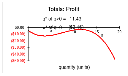
Figure 12.4: Case 3: Negative profits, continuing production.

Source: OutputProfitMaxPCSR.xls!Graphs.

The canonical graph of profit maximization can be used to determine whether the firm should produce or shut down by comparing price to average variable cost. The Shutdown Rule is easy: hire no labor and produce nothing if \(P < AVC\).

STEP Look at the bottom left graph on your screen. It confirms that the Shutdown Rule works. Profits are negative because price is below average total cost, but the firm will continue production because \(P > AVC\). When the relationship between P and AVC is such that price is greater than average variable cost, it means that the top of the profit function is higher than the y intercept, as in Figure 12.4.

STEP Click on the pull down menu (over cell R5) and select the Neg Profits, Shutdown option. Figure 12.5 displays the top right graph.

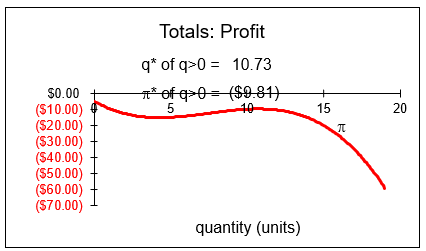
Figure 12.5: Case 4: Negative profits, shut down.

Source: OutputProfitMaxPCSR.xls!Graphs.

In this case, the top of the profit function is below the y intercept. In other words, the maximum profit if the firm produces, \(-\$9.81\), is worse than the negative profit incurred if the firm shuts down, \(-\$5\). The firm optimizes by choosing \(q \mbox{*}\) = 0, that is, shutting down.

STEP Look at the bottom left graph on your screen. Once again, we have confirmation of the Shutdown Rule. With P = 4.5, \(P < AVC\) and the firm should shut down.

STEP Carefully watch the canonical (bottom left) and profit function (top right) graphs as you change the price (with the pull down menu over cell R5).

As long as \(P > AVC\), the top of the profit hill is above the y intercept. If \(P = AVC\), the two are exactly equal and the firm is indifferent between producing and shutting down.

\(P < AVC\) is the magic cutoff point. When this happens, the top of the hill is below the y intercept (which is the negative profit suffered if the firm produces nothing). Thus, the firm’s best choice is to produce nothing.

Here is why the rule works. Multiply the Shutdown Rule by q to get: \[\begin{gathered} %star suppresses line # (P<AVC)q \\ Pq<AVCq\\ TR<TVC\end{gathered}\] \(TR<TVC\) is a restatement of the Shutdown Ruleproduce nothing if total revenue cannot cover total variable costs. This makes sense. Why produce if you can’t even pay for the variable expenses? You are better off not producing at all.

If total revenue is less than average total cost, then profits are negative. However, the firm can be in a situation where \(TR < TC\), but \(TR > TVC\). If so, then production makes sense because you will be able to reduce some of the fixed costs you have to pay no matter what you do. Profits are negative, but it is better to produce than not produce because variable costs are covered and fixed costs are at least partially reduced.

STEP For a summary of the four cases and what the Shutdown Rule is doing, click the button (over cell AC5).

What’s Normal about Zero Profits?

In economics, zero profits are called normal profits. This is confusing. Zero sounds bad, not normal. There is a logical explanation, but it requires a clear separation of accounting versus economic profits. They differ because economists include opportunity costs when calculating economic profits.

• Accounting profits = revenues - explicit costs
• Economic profits = revenues - explicit costs - opportunity costs

In economics, without an adjective, "profits" means economic profits. So, when profits are zero that means economic profits are zero. Economic profits have had an extra item subtracted, the opportunity costs of using firm resources to make this particular product.

An accountant would subtract explicit (out-of-pocket) costs (wages, rent, etc.) from revenues and if this number is positive, announce that the firm is making money. The economist would then subtract the cost of the profits that could be made by the next best alternative industry that the firm could be in. If economic profits are zero, it means the opportunity costs are exactly equal to the accounting profit and the firm cannot do better by switching to its next best alternative.

Although this may seem needlessly contorted at first, there is a nice interpretation of economic profits: If positive, the firm will stay in the industry and new firms will enter in the long run; if negative, the firm will exit in the long run; and if zero, there will be neither exit nor entry in the long run. It is in this sense of equilibrium that we say zero profits are normal. With \(\pi = 0\), there is stability and no tendency to change in the movement of firms.

The distinction between economic and accounting profits also explains why positive profits are excess profits. It is not meant as a pejorative term, but to indicate that the firm is earning greater profits than are needed to keep producing that product in the long run. Excess profits also mean that others are attracted and will enter that industry.

Economists are not concerned with how much money the firm made, but with profits as a signal to entry and exit. Defining economic profits as accounting profits minus opportunity costs gives us a profit measure that tells us whether the firm will stay or leave in the long run.

Shutdown Rule and Corner Solution

The Shutdown Rule is usually covered in introductory economics. Memorization is often all that is achieved. We can do better by properly situating the Shutdown Rule in the landscape of mathematical and economic conceptsit is a corner solution.

Recall that, in the Theory of Consumer Behavior, there are situations in which the MRS does not equal the price ratio, yet the solution is optimal. This is a corner solution.

Food stamps are an example. The fact that food stamps can only be used to buy food creates a horizontal segment on the budget constraint so that a consumer might not be able to make MRS = \(\frac{p_1}{p_2}\). At the kink in the constraint, the consumer is optimizing even though the equimarginal condition is not met.

Corner solutions are a general phenomenon. They can be seen whenever a restriction or border blocks further improvement in the objective function. Consider Figure 12.6 which sketches a maximization problem to highlight the difference between an interior and a corner solution. In panel B, the agent cannot choose negative values of the x variable and, therefore, the function is cut off by the y axis.

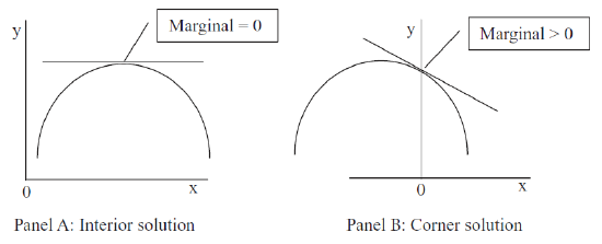Figure 12.6: Understanding the corner solution.

In panel B, although the marginal condition is not met, we have an optimal solution, defined as doing the best we can without violating any constraints.

Shutting down is another example of a corner solution because, once again, the equimarginal condition is not met at \(q=0\), yet producing nothing is the optimal solution. Shutting down is an unusual example of a corner solution because there is a place where the marginal condition is met (there is an output where \(MR = MC\)), but it is not optimal. The profit function twists in such a way (see Figure 12.5) that profit is decreasing as output rises from zero. This means that profits would go up if we were able to produce negative output. Since we are not allowed to choose \(q < 0\), we have a corner solution.

How can we know if we should choose q at \(MR = MC\), the interior solution, or shut down, the corner solution? The only way is to compare the profit positions at the two quantities. The good news is that no checking is required for cases 1 and 2. As long as profits are non-negative, there is no way that a profit of minus total fixed cost can be better than the interior solution of q where \(MR = MC\). But, whenever, \(MR = MC\) yields negative maximum profits, comparing those negative profits to TFC is necessary. Or, you could just use the Shutdown Rule and see if P < AVC, which will give the same, correct answer.

The complexity of the firm’s profit maximization problem in the short run, with its shutdown possibility, should increase your sensitivity to lurking problems with analytical and numerical methods. We know neither is perfect so there may be glitches in applying these methods to the firm’s profit maximization problem. The Q&A sheet provides an example. Be sure to look carefully at questions 2 and 3.

Finding and Displaying the Initial Solution

The output profit maximization problem for a PC firm in the short run is a single-variable (q) unconstrained problem. It can be solved with numerical and analytical methods. The equimarginal rule applied is that \(MR = MC\) and since price taking behavior means that \(P=MR\) for a PC firm, the equimarginal rule is often shown as \(P=MC\).

The firm’s profit maximization problem contains a complication in the short run. If maximum profits are negative, it is possible that the firm is better off not producing anything. A shortcut to determine whether or not to produce when \(\pi \mbox{*}<0\) is the Shutdown Rule, \(P < AVC\).

The initial optimal solution is displayed by a canonical graph that superimposes the firm’s revenue side (average and marginal revenue) over its cost structure (average and marginal costs). Optimal output is easily found where MR intersects MC (as long as \(P > AVC\)) and maximum profit is displayed as the area of the appropriate rectangle. The ability to instantly show the optimal solution, maximum profits, and whether or not to shut down explains the popularity of this graph.

You can think of the firm as walking through a series of three steps when solving its profit maximization problem:

1. Choose q where \(MR = MC\) in the canonical graph.
2. Compute profits at \(q \mbox{*}\) via \((AR - ATC)q\) (the profit rectangle).
3. If profits are negative, shut down if \(P < AVC\).

The PC firm’s profit maximization is simpler in the long run. If \(\pi < 0\), firms exit the industry; \(\pi > 0\) (also known as excess profits) lead to entry. Thus, in long run equilibrium (a state never actually attained), \(P = ATC\) and \(\pi = 0\) for all firms. This is why zero economic profits are called normal profits.

Exercises

1. Use Excel’s Solver to find the optimal output and profit for a firm with cost function \(TC = 2q^2 + 10q + 50\) and \(P = 40\). Take a screen shot of your optimal solution (including output and profits) and paste it in a Word document.
2. Use analytical methods to solve the problem in the previous question.
3. For what price range will the firm in question 1 shut down? Explain.
4. If fixed costs are higher, will this influence the firm’s shutdown decision? Explain.

References

The epigraph is from the foreword (p. vi) of Joan Robinson, The Economics of Imperfect Competition (first edition, 1933, followed by many reprints). In a male-dominated profession, Joan Robinson established herself as a well-known, important economist. She helped create the Theory of the Firm, including the canonical graph with average and marginal revenue and cost that is used to this day.

Ironically, however, much of her work was critical of mainstream economics. Her famous Richard T. Ely lecture at the 1971 American Economics Association conference pulled no punches:

For once the president of the AEA was a dissident. This was the veteran institutionalist and Keynesian John Kenneth Galbraith, a longtime friend of Robinson’s and celebrated critic of US capitalism and its apologists in academic economics. Galbraith now offered her the most important platform she had ever occupied. Robinson took full advantage of it, delivering an abrasive, challenging, deliberately provocative indictment of neoclassical economics that was designed to polarize her audience between the old and conservative and the young and progressive. (John Edward King, A History of Post Keynesian Economics Since 1936 (2002), p. 123.)