17.7: Cartels and Deadweight Loss

We know that the equilibrium output of a competitive market equals the output that maximizes consumers’ and producers’ surplus. We also know that monopoly produces too little output and the resulting deadweight loss is a measure of the inefficiency of monopoly. But competition and monopoly mark opposite ends of a spectrum that includes a wide range of other market structures.

A cartel is a type of market structure in which a group of firms cooperate to control output and price. Perhaps the most famous international cartel is the Organization of the Petroleum Exporting Countries, OPEC. Cartels are not monopolies because there are several independent firms in the syndicate or trust, but they hope to act like a monopolist, restricting output and raising price, to earn monopoly profits. Cartels are inherently unstable because it is in the interest of each member to cheat and sell more than the agreed amount.

This section explores the welfare properties of a specific type of cartel. The application is based on the workings of the Norwegian cement cartel as explained by Röller and Steen (2006). Analyzing the cartel involves solving a two-stage game and the cartel result is compared to monopoly and non-cooperative, Cournot competition. This material is advanced and it is recommended that the chapter on Game Theory be completed before proceeding.

A Brief History of Norwegian Cement

Cement output in Norway (and in other countries that use the metric system) is measured in tonnes (pronounced tons). This is not simply a foreign spelling for a ton. A ton is 2,000 pounds. A tonne, sometimes called a metric ton, is 1,000 kilograms. Given there are roughly 2.2 kilos in a pound, a tonne is about 2200 pounds. Thus, a tonne is bigger than a ton.

Figure 17.29 shows that production rose dramatically during the second half of the 1960s, greatly outpacing demand. This excess output was sold at a loss in other countries. A balance between production and consumption was restored by the early 1980s.

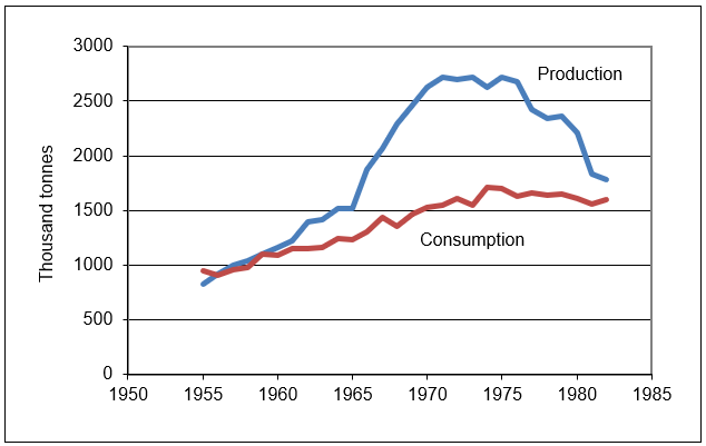
Figure 17.29: Norwegian cement production and consumption, 1955-1982.

Source: CartelDWL.xls!Data.

Production rocketed because of the sharing rule adopted by the Norwegian cement industry. A sharing rule determines how the monopoly rent is to be distributed among the firms in the cartel. Each firm’s share of the domestic market was based on its fraction of total industry capacity. We will see that this gives each firm an incentive to expand plant capacity and led to the explosion in output shown in Figure 17.29.

In 1968, the three producers in the cement industry abandoned the cartel market structure and merged to form a monopoly. By then, however, plant capacity had been expanded and it took years to reduce output.

Röller and Steen explain that there are few empirical studies of cartels because they are illegal in many places (including the United States) so obtaining data is difficult. Such is not the case in Norway. “Given the legality of the Norwegian cement cartel, we have a large amount of primary data allowing us to do a complete welfare analysis.” (Röoller and Steen, 2006, p. 321.

Monopoly Review

STEP Open the Excel workbook CartelDWL.xls, read the Intro sheet, then go to the Monopoly sheet.

Given the linear inverse demand curve and constant marginal cost, finding the monopolist’s profit-maximizing solution is easy.

STEP Use the scroll bar under the chart to find \(Q \mbox{*}\). As you change the quantity, you can see the corresponding price in the chart and in cell B11. You can also see the producers’ surplus (also known as profits) change in cell B19 as you set Q.

You can choose \(Q \mbox{*}\) by watching cell B19, but you could also find \(Q \mbox{*}\) by choosing the intersection of MR and MC.

Excel’s Solver offers yet another alternative to finding the profit-maximizing level of output.

STEP Run Solver and configure the Solver dialog box to solve the monopolist’s profit maximization problem.

Finally, click on cells B18, B19, and B21 to show the consumers’ surplus (CS), producers’ surplus (PS), and deadweight loss (DWL) from the monopoly solution in the chart.

Having found the monopoly solution, we turn to output (and price) under a noncooperative, Cournot environment.

Cournot Review

STEP Proceed to the CournotFirm sheet.

Chapter 16 on game theory presented the material reviewed here, which assumes a basic understanding of the Cournot model and Nash equilibrium.

Instead of a single firm, there are three firms making a homogeneous product. They do not collude or combine forces. Instead, they compete. Unlike perfect competition, however, there are so few producers that they impact each other’s decision making. If one firm decides to produce a lot, this will lower the price for all three firms.

How will an individual firm decide how much output to make? The core idea is that each firm will make profit-maximizing output decisions based on conjectures about what the other firms will do. The output level at which each firm’s decision is consistent with the output chosen by the other firms is the solution, called a Nash equilibrium.

The CournotFirm sheet opens with cell B10 set equal to zero. This means that Firm 1 is exploring what its best option is if the other firms produce nothing.

STEP Use the scroll bar under the chart to find the profit-maximizing output for the conjecture that the other firms produce nothing.

If the other firms decide to produce zero output, Firm 1 will produce 2.3 million units of output. But this is not an equilibrium solution because the other firms would not choose to produce zero units of output when this firm produced 2.3 million tonnes. How much would the other firms produce?

STEP Click the button to copy Firm 1’s optimal solution (in cell B15) to the conjectured output in cell B10.

Notice how the chart shows new red D and MR curves. These are the residual demand and residual marginal revenues curves for Firm 2, given that Firm 1 produces 2.3 million and Firm 3 produces nothing.

STEP Use Excel’s Solver to find the profit-maximizing output for the conjecture that the other firms produce 2.3 million units.

You should find that Firm 2 will produce 1,150,000 units when the other two firms produce 2.3 million. We have stumbled upon the Nash equilibrium solution! If each firm produces 1.15 million units, then none of them will regret its output decision. In other words, each firm’s optimizing decision (1.15 million) is consistent with the conjectured output (2.3 million).

Notice that the Nash equilibrium is not Firm 1 = 2.3 million, Firm 2 = 1.15 million, and Firm 3 = 0. Both Firms 1 and 2 would regret their decisions and would opt for different output choices. It should be clear, however, that if each one makes 1.15 million, then none of the firms would regret or wish to change its chosen output level.

The Cournot solution can be found via iteration (which was easy in this example) or by analytical methods (see work starting in cell A28). The reduced form for the industry’s Nash equilibrium output in this Cournot model (linear demand and cost function and n firms) is: \[Q_e=\frac{n}{n+1}\frac{d_0-MC}{d_1}\] Price, of course, is simply read from the inverse demand curve.

STEP Proceed to the Cournot sheet to see the welfare implications of the Cournot solution. Click on cell B14 to see that the formula for the Nash equilibrium has been entered.

Notice that the Cournot output level is between the perfectly competitive (\(D = MC\)) and monopoly (\(MR = MC\)) output levels.

STEP Click on cells B18, B19, and B21 to highlight CS, PS, and DWL in the chart.

Once again, notice that the DWL for the Cournot solution is between the monopoly (highest DWL) and perfect competition with many firms (no DWL) extremes.

STEP Increase the number of firms in cell B10 to 5, 10, and 20.

As n rises, DWL falls because as n rises, we are approaching the ideal solution of competition with many firms. Thus, perfect competition is simply an n-firm Cournot model with an infinite number of firms. You can confirm that at \(n = 1\), the monopoly solution is found.

Having covered the monopoly and competitive Cournot models, you are ready to tackle yet another market structure: the cartel.

Cartel Behavior

Suppose an industry, made up of several firms, organized into a cartel. In other words, the firms would join forces and cooperate in making decisions. The cartel would decide the total domestic output and price for the product. In addition, the cartel would have to determine how much each firm would produce. This is called the sharing rule.

Different sharing rules yield different results. Suppose that the sharing rule applied is that each firm’s output reflects its share of total industry capacity. There are no limits on each firm’s capacity and any output not sold domestically could be exported at the world price.

Although each firm chooses capacity first and then the cartel chooses total output (and price), we solve the two-step optimization problem recursively. This means we start at the second stage, then work backwards to the first stage.

Stage 2: Choosing Total Domestic Output (and Price)

STEP Proceed to the CartelStage2 sheet.

The information is laid out as in the Monopoly sheet, but there are additional variables. The world price (below marginal cost) has been added in cell F8 and to the chart. Individual firm parameters start in row 26. The three firms have chosen their capacities (cells B30:B32), determining total capacity (B28) and shares of domestic output (C30:C32).

STEP Use the scroll bar under the chart to explore different quantities of domestic output. This is the cartel’s key choice variable. It can choose anywhere from no output to the vertical, total capacity, line (which is determined by the firm’s capacity decisions in stage 1 and is now an exogenous variable to the cartel).

STEP Click on cell B19, which is the PS and also the profit generated by a given output level, to highlight the PS in the chart. The formula and the chart reveal that PS has two parts: = (P \(-\) s0_)*Q \(-\) (s0_ \(-\) R_)*(B28 \(-\) Q).

The first part is a rectangle with height from MC to price and width from zero to the chosen output. This would be PS under monopoly.

But the cartel has a second component to PS. This is the smaller rectangle on the chart and it is subtracted from the bigger rectangle. This second part is the excess output that is exported and sold at the world price. It is subtracted from profits because the world price is below MC. Thus, these units are sold at a loss.

STEP Use the scroll bar to find the cartel’s \(Q \mbox{*}\). Notice that you can find the optimal output by keeping an eye on PS (in cell B19) or by setting \(MR = R\). You can also use Excel’s Solver to find the optimal output.

Cell B13 shows the optimal output and your cell B12 should equal this solution. The cartel will produce 3,150,000 units and charge $1,725 per unit. This is a higher output (and lower price) than the monopoly solution.

R is a key variable. It plays the role of MC in the cartel’s optimization problem. What effect does changing R have on \(Q \mbox{*}\) and \(P \mbox{*}\)? What welfare effect does changing R have? We can answer these questions with Excel.

STEP Change R to 500 in cell F8. Solve the cartel’s optimization problem again.

You should see that optimal domestic quantity is lower and price is higher.

STEP With the new optimal solution for \(R = 500\) in B12 (\(Q \mbox{*}\) = 2.8 million), click the button. It displays the initial CS, PS, and DWL values (for \(R = 150\)) and computes the difference between the new and initial values.

As R rises, CS falls and PS rises. Total DWL is bigger by $136 million, with both parts of DWL (the traditional triangle that represents domestic DWL and the export loss) rising.

STEP Click the button (or reset R to 150).

We conclude our analysis of the cartel’s first stage of the optimization problem by examining the effect on the individual firms. Cells D30:G32 show how the sharing rule is applied to determine how much each firm produces, given the cartel’s total domestic output decision. The blue text color means these variables are endogenousthey are determined by the cartel’s domestic output decision.

STEP Adjust Q via the scroll bar under the chart and keep your eye on cells D30:G32. As Q changes, so do the individual firm variables in blue.

Because the firms have equal capacities, each sells a third of the domestic output and exports the rest. Domestic and export sales for each firm are displayed.

STEP Enter 3,150,000 in cell B12 (the value of \(Q \mbox{*}\) at the initial values of the exogenous variables) to see the PS earned by each firm at the cartel’s optimal output.

From the cartel’s point of view, the individual firm capacities are given. But would profit-maximizing firms choose these particular capacities? This question is at the heart of the first stage of the cartel’s two-stage optimization problem.

Stage 1: Choosing Capacity

Now that we know how the cartel is going to decide how much domestic output to produce and the sharing rule, we can tackle the question facing each firm: How much capacity?

At any point in time, firms have a given maximum total production, or capacity, determined by factory size. To increase capacity, firms must expand factory size and this takes time.

Notice that the marginal cost of cement production is different from the marginal cost of capacity. The former is assumed to be low and it does not play a role in this analysis. In fact, it is assumed that firms always produce up to capacity.

The capacities of each firm and hence total capacity are given to the cartel but are chosen by each firm. Each firm would pick that capacity that would maximize its profits.

The profit function has revenue from two sources: domestically sold output at price P (chosen by the cartel) and the excess output that is exported and sold at the world price, R. The cost of capacity function is linear, with constant marginal cost.

STEP Proceed to the CartelStage1 sheet and click on cell B11 to see that the formula reflects the firm’s profit function.

Cells B19:B23 have the exogenous variables. Each firm chooses capacity (\(q_i\)) to maximize profits.

The sheet opens with the firm having a capacity level of 1,200,000 units, the same as the other two firms, so the total industry capacity is 3,600,000 units.

STEP Click on the scroll bar (next to B27) to increase capacity.

Notice that the larger the chosen capacity, the greater the share of the domestic sales (Q), which is chosen by the cartel, and thus domestic revenues (B13) rise. As capacity increases, exports also rise (because only a share of the firm’s output is sold domestically) and this hurts because the world price is below marginal cost. Of course, increasing output is going to increase costs because the firm has to build a bigger plant.

Given these trade-offs, what level of capacity should this firm select?

STEP Keep your eye on cells F27:H27 as you adjust the scroll bar to select the profit-maximizing output.

As usual, you can equate MR to MC to find the optimal solution.

STEP Check your work by using Excel’s Solver.

The optimal capacity, 1,342,758 units, differs from the original 1.2 million units. This means that the optimizing firm would choose to make 1,342,758 units when the other two firms make a total of 2.4 million.

STEP Copy the optimal capacity in cell B27 and paste it in cell K9 (or enter 1,342,758 units in cell K9).

We are not done yet because if this firm wants to make 1,342,758 units, it stands to reason that the other firms (with identical cost structures) will also want to do this.

STEP Return to the CartelStage2 sheet, select cell B30, and paste (or type in) 1,342,758.

Notice that cells B31 and B32 change to the value of cell B30. Cell B28, Total Capacity, is now higher and, thus, the vertical line in the chart has shifted right.

We do not need to run Solver again because the cartel’s optimal output and price combination in the domestic market is unaffected by the total industry capacity. The extra output is simply exported and sold at the world price.

STEP Return to the CartelStage1 sheet and notice that MR no longer equals MC. Click on cell B20 to see that it has a formula.

Cell B20, Other Capacity, has changed because the other two firms have selected different capacities.

STEP Copy cell B20, select cell J10, and Paste Values, then run Solver. Copy the new optimal Q (cell B27) and paste it in cell K10.

Notice that we still do not have an internally consistent solution between the two optimization problems. The firm capacity optimal solution is different from the total capacity used by the cartel. We must iterate.

STEP Do these three steps:

1. In the CartelStage2 sheet, select cell B30, and paste the value of optimal capacity.
2. Return to the CartelStage1 sheet and copy cell B20, select cell J11, and Paste Values.
3. Run Solver to find the new optimal solution. Copy the optimal Q (cell B27) and paste it in cell K11.

We still do not have a situation in which the optimal capacity decision of Firm 1 agrees with the total capacity parameter used by the cartel.

STEP Fill in the Stage 1 and Stage 2 Consistency table. You will need to iterate, repeating the process of solving for Firm 1’s optimal capacity, pasting that result in the CartelStage1 sheet, then returning to the CartelStage2 sheet to see if the two solutions coincide (the three steps above).

STEP When you have finished completing the table, click the button.

This reveals results in columns L, M, and N that are based on your iterations. It also shows the Nash equilibrium solution for \(q_i \mbox{*}\). As with our work in the Cournot model earlier, there is an analytical solution to each firm’s optimal and consistent capacity and we entered it in cell K19.

Figure 17.30 shows what your screen should look like. The total capacity, the vertical line in the CartelStage2 chart, is driven to an equilibrium value of 3,891,176 units. The total capacity line bounces right and left until settling down at a value that is consistent with the optimal solution to the individual firm’s profit maximization problem. In equilibrium, each firm will have a capacity of 1,297,059 units. This is consistent in the sense that each firm would choose this capacity if it knew the sharing rule adopted by the cartel.

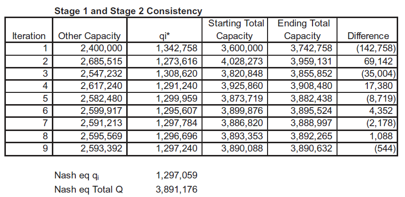
Figure 17.30: Nash Equilibrium capacity.

Source: CartelDWL.xls!CartelStage1.

Given the demand curve parameters, marginal cost, and the world price, we know the cartel’s profit-maximizing domestic output and price. Because we know the equilibrium solution to each firm’s capacity decision, we can compute the total output produced and export loss. Thus, we can compute CS, PS, and DWL.

STEP Copy cell K19 from the CartelStage1 sheet and Paste Values in cell B30 of the CartelStage2 sheet.

STEP Click on cells B18, B19, and B21 to display the CS, PS,and DWL generated by the cartel solution.

Cartel Model Summary

Determining the cartel’s output is not easy. One has to solve a two-stage game. The cartel’s sharing rule means that each profit-maximizing firm is willing to trade off export losses in order to get a share of high-priced domestic output.

The vertical total capacity line in the CartelStage2 chart is actually an equilibrium solution to the first stage of the game. There is only one value of total capacity that is internally consistent with individual firm capacity decisions.

The cartel game-theoretic model also can be solved via analytical methods. The mathematics is not easy, but if you are interested in seeing the solution, click the button near cell M5 of the CartelStage1 sheet.

Having determined the output and price solutions to each of the three market structures, we are ready for the welfare analysis.

Comparing Monopoly, Cournot, and Cartel Solutions

STEP Proceed to the Compare sheet.

Given the parameter values (in the shaded cells), the table displays the output, price, CS, PS, and DWL associated with perfect competition, monopoly, cartel (with the sharing rule), and Cournot market structures.

Cells B18:B21 are connected to the market structure currently displayed on the chart. Initially, the perfectly competitive result is displayed. DWL will be computed against this standard.

STEP Click the Monopoly option.

Cell range B18:B21 is updated and the chart displays the monopoly result. Notice that the monopolist ignores the world price and does not export cement. She maximizes profits by choosing output where \(MR = MC\).

Compared to perfect competition (in cells B10:B14), monopoly generates much lower CS, higher PS, and a substantial DWL.

STEP Click the Cartel option.

The chart displays the total capacity vertical line and the exports are highlighted. We can compare the cartel to the monopoly and PC results by looking at the cells in columns B, C, and D, in rows 10 to 14.

Note that for the cartel option, cell D13 shows the value of profits for the cartel. This is domestic PS less export loss. Cell B19, also labeled PS, shows domestic producers’ surplus (and leaves out the export loss). This is confusing, but it allows separation of the two sources of total DWL, domestic DWL, given in B21, and export loss, shown in cell B22, and ensures that domestic DWL plus total surplus will sum to total surplus in the perfect competition case. Total DWL, the sum of domestic DWL and the export loss, is reported in cell D14.

Compared to perfect competition, the cartel generates lower output and higher prices, but it is better than monopoly. Cells G10:G14 show what happens when you move from cartel to monopoly.

STEP Click on cells G10 to G14 to see their formulas.

If the Norwegian cement industry merged to monopoly from a cartel, we would see the following: Output falls, price rises, CS falls, PS rises, and DWL rises.

The increase in DWL would enable to us to judge such a move as a failure in terms of resource allocation in the Norwegian economy.

STEP Click the Cournot option.

Comparing cartel and monopoly to perfect competition is not particularly useful, because we are not going to get a perfectly competitive cement industry. There are only three firms. If we had competition, it would be Cournot competition. The three firms would not collude, but they would behave strategically.

If the industry went from cartel to Cournot, cells F10:F14 show what would happen. As with cells G10:G14, these cells report the difference from the cartel to the Cournot market structure. Notice that output rises, price falls, CS rises, PS rises, and DWL falls.

Of these effects, PS rising is surprising, but remember that under Cournot, the export losses are eliminated.

This completes the theoretical welfare analysis. The results are clear: To maximize surplus, the Norwegians should have moved from a cartel to Cournot competition. Of the three market structures, Cournot has the lowest DWL.

There is, however, one important issue left unresolved: These results apply only to the parameter values on the sheet. We do not know the intercept or slope of the Norwegian demand curve for cement, nor do we know R or MC. We need to get these parameter values, and then do the analysis based on these real-world parameter values.

Welfare Analysis for 1968

STEP In the Compare sheet, scroll to the right of the graph and click the button (over cell N1).

After clicking the button, a new sheet appears, populated with key parameters for 1968, the last year of the cartel.

Figure 17.31 shows the results for the various market structures for the estimated demand curve for 1968. The conclusion is clearCournot is the best of the three feasible market structures. It produces the highest output, lowest price, highest CS, and lowest DWL.

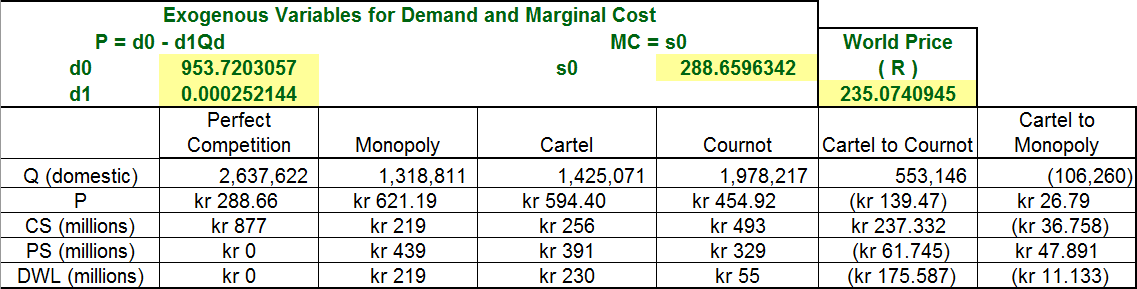
Figure 17.31: Welfare analysis.

Source: CartelDWL.xls!CompareActual.

Figure 17.31 also makes clear why the industry went to monopoly instead of Cournot after the cartel collapsed (under the weight of overproduction and export losses). PS would rise when moving from Cartel to monopoly (by 47,891,000 kroner), but fall (by 61,745,000 kroner) if the industry had adopted a noncooperative Cournot arrangement. Thus, it is clear that the cement industry chose to maximize its own PS instead of \(CS + PS\). This is not surprising.

In fact, Röller and Steen build an even stronger case by exploring the welfare effects over several years. Scroll to column AE and read the text box if you are interested.

STEP Click the Monopoly option to display the monopoly solution in the graph.

The monopolist would choose output where \(MR = MC\) and charge the highest price possible for that level of output. Monopoly profit in 1968 would have been 439 million kroner. Consumer surplus would be much smaller than under perfect competition and Norway would suffer a deadweight loss from monopoly of 219 million kroner.

But the Norwegians did not have a monopoly before 1968, they had the cement cartel.

STEP Click the Cartel option.

The cartel chooses output where \(MR = R\), allocates the domestic output to the three firms based on capacity shares, and exports the excess output.

Notice, however, that Röller and Steen do not use the predicted capacity based on the demand curve parameters. Instead, they use actual exports. The story here is that capacity takes time to build. The cartel puts persistent pressure on expansion, but the firms do not actually reach their goal of vast capacity because the cartel collapses.

STEP You can check the theoretical cartel solution for the estimated parameters by simply copying the range A5:F8 from the CompareActual sheet and pasting in the same range in the Compare sheet. Click Yes if prompted to replace the destination cells. You may need to click the Cartel option to refresh the screen.

Figure 17.32 shows the result. Capacity is huge and export losses are staggering. This is the capacity that would have been installed in the long run under the cartel. Röller and Steen do not use this capacity value. Instead, they use actual exports, based on the actual capacity in 1968.

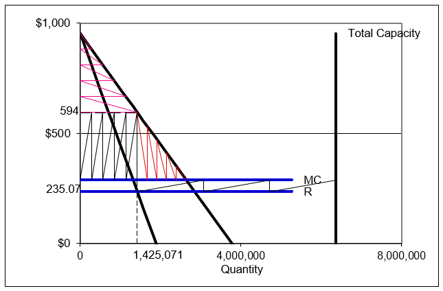
Figure 17.32: Cartel results with capacity determined theoretically.

Source: CartelDWL.xls!Compare using estimated parameters for 1968.

STEP Return to the CompareActual sheet. Focus on columns F and G.

We know the firms merged to monopoly and the cartel to monopoly column (G) shows the welfare implications of this move for just 1968. As expected, output falls and price rises, CS falls and PS rises. The net welfare effect can be computed as the sum of the changes in CS and PS, which is an 11 million kroner increase (in cell G15).

Alternatively, the net welfare effect can be determined by looking at the reduction in DWL in cell G14. Because DWL falls as we move from cartel to monopoly, this number is negative. But notice that the absolute values are the same.

Our standard models tell us that merger to monopoly is the worst possible outcomemonopoly generates the greatest DWL of any market structure. However, because of the sharing rule, welfare actually increases when the cartel merges to monopoly because monopoly does not suffer export loss.

STEP Compare the values in Table 3 for the cartel to monopoly in 1968 to the values in column G.

The slight differences are due to rounding and precision differences.

Although monopoly beats the cartel, this is a poor argument for supporting monopolization. After all, the cartel could have dissolved into a noncooperative, Cournot competition. We must examine the welfare effects of this move and compare it to moving to monopoly to find the better option.

STEP Compare the red circled value of the change in PS when moving from Cartel to Cournot in Table 3 to cell F13. These numbers should be the same, but they are not.

Röller and Steen made a mistake in computing the net welfare effect for the move from cartel to Cournot in Table 3. They report the change in domestic PS in the table, not the change in total PS, which includes the export loss. As a result, the net welfare effect for cartel to Cournot in Table 3 is also incorrect. By failing to include the export loss in the reported PS, they underestimated the welfare gain from adopting a Cournot noncooperative market structure.

This error does not change Röller and Steen’s conclusion. In fact, if anything, their results are strengthened once the export loss is accounted for. The loss in PS that the cement industry undergoes in moving to Cournot competition is not as bad as Table 3 suggests because of the elimination of the export loss. The true net change in welfare is some 45 million kroner higher than Table 3 estimates.

Consequences of Using Actual Versus Theoretical Total Capacity

Now that we understand how net welfare effects for 1968 are computed, we turn to the issue of how the export loss is measured.

Cell D20, the export loss in 1968, is based on actual exportsthe difference between actual capacity (total production) and domestic output.

Figure 17.32 and your Compare sheet show that at the Nash equilibrium, long run capacity is much higher than the actual capacity (based on actual total production). How does this impact the analysis? This is an important question with a surprising answer.

STEP Compare the formulas in cells G16 and G17. Both display the same number, but the formulas are different.

G16 computes the net welfare gain from going to Cournot instead of monopoly (from the cartel, of course) by taking DWL from cartel to Cournot minus the DWL from cartel to monopoly. Cournot beats monopoly by about 165 million kroner.

G17 computes the same net welfare gain, but does so by subtracting the net welfare effect from going to monopoly from the net welfare effect from going to Cournot. Once again, the move to Cournot beats the move to monopoly by roughly 165 million kroner.

STEP Copy the two cells, G16:G17, and go to the Compare sheet, pasting these cells in the same range.

The result is surprisingthe superiority of Cournot over the cartel remains exactly the same, even though the Compare sheet is using theoretical, long run total capacity and the export losses are huge.

If you compare the values in columns F and G in both sheets, you will find that for both the move to monopoly and the move to Cournot, the change in PS and the change in net welfare are much higher if the theoretical capacity is used. This makes sense because the export loss is much greater.

However, the relative improvement in Cournot over monopoly remains the same because both Cournot and monopoly avoid export losses. Thus, the size of the export loss does not matter.

Had Röller and Steen used the theoretical, long run total capacity level based on the estimated parameters in 1968, their qualitative and quantitative conclusion regarding the superiority of Cournot over monopoly would remain completely unaffected.

Lessons from the Norwegian Cement Cartel

Röller and Steen (2006) evaluate the effectiveness of the (legal) cement cartel in Norway over the period 1955 to 1968. They solve monopoly, Cournot, and cartel models and compare the results. They find that because of the sharing rule adopted by the cartel, consumers actually did better (in terms of consumer surplus) than they would have if the industry had been monopolized. Producers, on the other hand, lose in the domestic market with the cartel compared to a monopoly. Producers suffer an additional export loss under the cartel and this leads to a key result: The merger to monopoly that occurred in 1968 actually improved net welfare relative to the cartel outcome. This is certainly a surprise, given that we expect monopoly to be the worst market structure. The authors point out, however, that simply breaking up the cartel and allowing Cournot competition would have improved welfare even more.

The fact that Röller and Steen used actual exports instead of estimated exports makes no difference to their final conclusion that Cournot competition would have been the first-best choice. The reason it does not matter is that both monopoly and Cournot competition result in the elimination of the export loss, so in comparing a move to either Cournot competition or monopoly, the actual size of the export loss is irrelevant.

Röller and Steen (2006) give an excellent example of how economists use CS, PS, and DWL in policy analysis. It also enables deeper understanding of game theory by examining the two-stage game played by members of the cartel.

This section is certainly not typical of an Intermediate Micro course, but it offers advanced students a chance to see a sophisticated application of welfare analysis.

Exercises

Suppose the inverse demand curve is \(P = 1000 - 0.5Q\), marginal cost is constant at $100 per unit, and the world price is $50. Enter these parameter values in the Compare sheet and answer the questions below. Enter the demand slope as a positive number, 0.5, and click one of the market structure options to refresh the chart.

The math theory prep section showed two surprising results. First, consumers’ and producers’ surplus under the cement cartel do not depend on the marginal cost of capacity. Second, as the number of firms in the cartel rises, the likelihood a merger to monopoly will be welfare enhancing rises.

To answer the questions that follow, taking pictures is helpful. You can select cells (e.g., A1:M25) and copy as a picture, then paste.

1. Increase MC from 100 to 200 and determine the impact on the cartel’s Q, P, CS, PS, DWL, and export loss. What happens to each of these variables as MC rises?

   Be sure to click the Perfect Competition and then Cartel option button to refresh the data below the buttons.

2. Which changes, if any, in the variables are surprising? Why?
3. At what value of MC will there be no exports? Take a picture of this situation and paste it in your Word document.
4. Increase the number of firms from 3 to 5 (with MC at the no export loss value). What effect does this have on the cartel’s Q, P, CS, PS, DWL, and export loss?
5. What can you conclude about the effect of the number of firms on PS from a merger to monopoly (from the cartel)?

References

The epigraph is from page 278 of Oliver E. Williamson, The Economic Institutions of Capitalism: Firms, Markets, Relational Contracting (1985). Williamson applies the standard tools of economic reasoning (optimization and comparative statics) to transactions and argues that the institutions we observe are the evolutionary product of selection based on optimization.

This application is based entirely on the excellent paper by Lars-Hendrik Röller and Frode Steen, “On the Workings of a Cartel: Evidence from the Norwegian Cement Industry,” American Economic Review, Vol. 96, No. 1 (January, 2006), pp. 321–338, www.jstor.org/stable/30034368. Special thanks to Frode Steen for making additional data available.