18.1: The Edgeworth Box

We have become quite familiar with society’s resource allocation problem. We have used partial equilibrium analysis to focus on a single commodity, exploring how supply and demand determine an equilibrium quantity that is the market’s answer to the resource allocation question.

We know all about consumers’ and producers’ surplus, market failure, and deadweight loss. We have repeatedly drawn supply and demand graphs and emphasized comparison of equilibrium to socially optimal output.

But the focus on a single commodity is limiting. In fact, the market system uses supply and demand for each good or service to answer the fundamental production and distribution questions. In other words, there are many interacting markets (one for each commodity) simultaneously in operation.

If we monopolize one commodity, we cause a misallocation of resources in the monopolized market (too little is produced). Partial equilibrium analysis stops there. But the low output and high price in the monopolized market reverberates throughout the economy. After all, resources that would have gone into that market are going to go somewhere else and the high price in the monopolized commodity will shift demand curves for substitutes and complements of that good.

General equilibrium analysis attempts to account for supply and demand in all markets at once. As you can imagine, it is much more difficult than partial equilibrium analysis, but it is also superior because the entire resource allocation question is under consideration.

This book focuses on general equilibrium theory, but as the epigraph to this chapter explains, computable general equilibrium models are used to estimate the general equilibrium effects of tax policies, monopoly power, and other events. Economists have always been aware of the limitations of partial equilibrium analysis, but it was not until the development of modern computers that these complicated models could be solved and applied.

Before beginning our study of general equilibrium theory, two observations are in order.

1. Society can decide which goods and services are handled by the market. Society may decide that human organs or votes may not be legally bought and sold. Different market-based societies may choose different lists of commodities to be allocated by the market. We call a society market based if individual resource owners make decisions about how to allocate the inputs they manage, even if particular commodities are regulated or entire sectors of the economy (such as education or health) are not privately owned.
2. A complete general equilibrium analysis of the market system is beyond our scope. There are three parts, of which this book covers only the first one.
   • Pure exchange: Assume each consumer has endowments of already produced goods and allow trade to occur.
   • Production: Allow goods to be produced from inputs.
   • Combine pure exchange and production in a general equilibrium analysis.

We focus solely on pure exchange and ignore the next two stages. This means we will not complete a true general equilibrium analysis of the market system. Emphasizing only the problem of pure exchange enables you to see the core concepts of general equilibrium, including the Edgeworth Box graph, without overwhelming complexity.

Even limiting ourselves to a situation where all products are already made requires serious investment of intellectual capital. As we will see, the Edgeworth Box is a clever graph, but it takes some practice to read it.

Our work on pure exchange will enable us to come full circle and return to the beginningconsumers decide what to buy and sell based on the optimal solution to an Endowment Model. As you work on the model and recall ideas and terminology, you will further cement truly fundamental knowledge.

Constructing the Edgeworth Box

The canonical graph used to depict a pure exchange economy is called the Edgeworth Box. It is also commonly referred to as the Edgeworth-Bowley Box. It turns out that both names are wrong. Blaug (1996, p. 523), discussing something called the Ricardo Effect, points out an interesting thing about names:

Whether it really is in Ricardo is a nice question. The fact that the Ricardo Effect is hard to find in Ricardo exemplifies a general rule. According to R. K. Merton, ‘eponymy’ is the “the practice of affixing the name of the scientist to all or part of what he has found” but it is a striking fact that the outcome of eponymy is almost always to hang the right label on the wrong person. Thus, Thomas Gresham never stated Gresham’s Law. Jean Baptiste Say only stated Say’s Law after James Mill had stated it for him. Robert Giffen never stated Giffen’s Paradox. Francis Edgeworth never drew the Edgeworth Box. Ernst Engel never drew an Engel’s curve. Walras never stated Walras’ Law. Irving Fisher did not invent the Ideal Index Number and actually pleaded (in vain) that it should not be named after him. Arthur Bowley did not enunciate Bowley’s Law. Arthur Pigou did not state the Pigou Effectand so on. Indeed S. M. Stigler has advanced “Stigler’s Law of Eponymy: No scientific discovery is named after its original discoverer,” a law which is confirmed as soon as it is stated (see Transactions of the New York Academy of Sciences, Series 11, 39, 1980). Nevertheless, there are also counter-examples in economics to Stigler’s Law, such as Pareto-optimality and the Wicksell Effect.

If it was not Edgeworth, then who created the canonical graph of general equilibrium analysis? According to Tarascio (1972), it was Vilfredo Pareto (pronounced pa-ray-toe) who should be credited with inventing the graph that we call the Edgeworth Box. Because no one has ever heard of the Pareto Box, we will continue to call it the Edgeworth Box, but now you know the truth behind the name.

The Edgeworth Box is a graph that is constructed by putting together the consumer choice problem graphs from two consumers. It ends up looking like a box; hence its name. While most books just draw a box, we can use Excel to see exactly how you build an Edgeworth Box.

STEP Open the Excel workbook EdgeworthBox.xls and read the Intro sheet, then go to the A sheet to see consumer A’s optimization problem.

Take the time to look over the sheet. The goal is to maximize satisfaction, given by a Cobb-Douglas utility function that faithfully reflects the consumer’s preferences. The budget constraint’s slope is \(-\frac{p_1}{p_2}\) and at the initial endowment (35,10), the MRS is less than the price ratio.

You know you do not need to run Solver because at 25,\(16 \frac{2}{3}\) (the actual values on the sheet are Solver’s false precision) the equimarginal condition is met and the consumer is reaching the highest attainable indifference curve.

At the given prices, the sheet shows that A will maximize utility, subject to the budget constraint, by selling 10 units of \(x_1\) and buying \(6 \frac{2}{3}\) units of \(x_2\). These are the net demands for \(x_1\) and \(x_2\).

STEP Proceed to the B sheet to see consumer B’s optimal solution.

Notice that B has a different initial endowment (5,30) than A, but the rest of the optimization problem is the same. Given the same prices faced by consumer A, consumer B optimizes by buying 20 units of \(x_1\) and selling \(13 \frac{1}{3}\) units of \(x_2\).

Figure 18.1 has Endowment Model graphs for the two consumers. We can see that they make different decisions about what to buy and sell. A moves up the constraint (selling \(x_1\) and buying \(x_2\)), while B does the reverse.

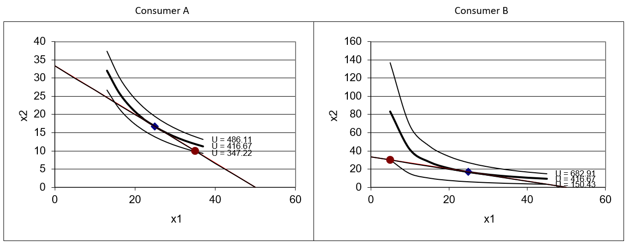
Figure 18.1: Preparing to build the Edgeworth Box.

Source: EdgeworthBox.xls!A and B.

Figure 18.1 shows the two consumers side by side and that helps us see what they are both doing, but it does not show how their plans for buying and selling match up. This is the key to the Edgeworth Box. We want to be able to instantly see if the two consumer’s optimal decisions mesh.

The crucial step in understanding the Edgeworth Box is the next one: Flip consumer B’s graph, as shown in Figure 18.2. Sheet B in Edgeworth-Box.xls shows how to do this.

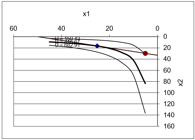
Figure 18.2: Flipping B’s graph.

Source: EdgeworthBox.xls!B.

STEP Follow the instructions in column F of sheet B to replicate Figure 18.2.

Actually flipping B’s graph will help you remember that B’s decisions about buying and selling are always read from the perspective of the northeast (top right) corner of the Edgeworth Box.

The last step in constructing the Edgeworth Box is to join A’s graph with B’s flipped graph. The result of this operation is a graph that looks like a box.

STEP Proceed to the EdgeworthBox sheet for your first look at an Edgeworth Box. You may need to scroll down a bit to see it.

How is this chart created? By following the instructions above and taking advantage of Excel’s ability to make transparent objects.

STEP Click on the graph to select it, and then drag the graph to the right.

It comes apart! Clearly, the Edgeworth Box is simply two separate graphs superimposed on top of each other. The top graph has no fill, so it is transparent.

STEP Click the button to put the box back together. The button simply lines up the two graphs precisely to make it easy to create the box.

STEP Scroll back up to see the organization of the sheet.

Let’s take a tour of the sheet. The two consumers’ optimization problems are represented in columns A and B and columns M and N. In the middle (columns G and H), market information is displayed. Cells H16 and H17 contain the prices of the two goods.

The price of good \(x_2\), called the numeraire, has been set equal to 1 and \(p_1\) is expressed as \(\frac{p_1}{p_2}\). Instead of \(p_1 = 2\) and \(p_2 = 3\), we can focus on \(\frac{p_1}{p_2}=\frac{2}{3}\) as the relative price. With many goods, a single one is chosen (think gold) as the numeraire and everything is priced relative to that good. In the next chapter, we will see how prices respond to supply and demand.

Properties of the Edgeworth Box

The Edgeworth Box has properties and conventions that will be helpful in our future work. Here are a few of them.

1. The sides of the box give the total amounts of the two goods available. Total \(x_1 = 40\) units and total \(x_2 = 40\) units so this box is a square.
2. If there is more total \(x_1\) than \(x_2\), then the box is wider than it is tall (if the same axis scale is used for both goods). The first exercise question asks what it means if the box is tall and skinny.
3. Since consumers face the same prices, one budget line is shared for both consumers.
4. The slope of the budget line is the price ratio, \(\frac{p_1}{p_2}\), and that is what matters, not the individual prices themselves. By convention, we normalize the problem and set \(p_2 = 1\), and call \(x_2\) the numeraire.
5. Net demands for \(x_1\) and \(x_2\) for both A and B can be read from the box. This requires careful attention because it is easy to be tricked. Remember to read B’s decisions about buying and selling from the top right corner.
6. The Edgeworth Box has enough information to figure out how prices will change and where the equilibrium solution lies. The next section shows how.

Edgeworth Box Basics

This section introduced the canonical graph of general equilibrium theory. It is unlikely that you have seen this graph before so we are proceeding slowly. Figure 18.3 shows the chart the EdgeworthBox sheet.

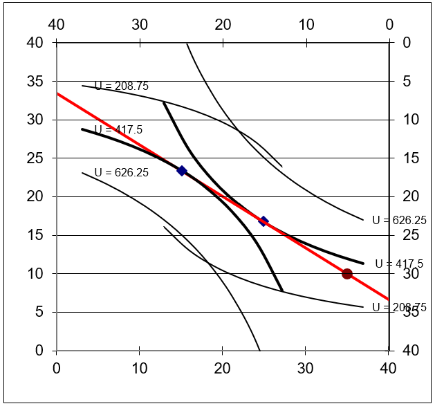
Figure 18.3: An Edgeworth Box in disequilibrium.

Source: EdgeworthBox.xls!EdgeworthBox.

The Edgeworth Box simultaneously displays the optimization problems of two consumers. A’s view is the usual x–y axis configuration with the origin in the lower left corner of the graph. B’s graph has been flipped so the origin is at the top right corner. Thus, \(x_1\) rises as you move to the left on the top of the box and \(x_2\) rises as you move down the right side of the box.

If you drew an Edgeworth Box on a piece of paper or are reading this on a laptop or tablet, you could literally rotate the paper or device so that B was the usual configuration at the bottom left and A’s axes were at the top and right. This would not change anything substantive.

In the next section, we will use the Edgeworth Box to see how both markets equilibrate simultaneously. This is the hallmark of general equilibrium analysis. Figure 18.3 is not in equilibrium. There are forces that will make the red budget line swing.

The Edgeworth Box will also be used to explain the concept of Pareto optimality and the idea of economic efficiency in a general equilibrium setting. Although it does not have the widespread recognition of supply and demand, the Edgeworth Box is a truly foundational graph in general equilibrium theory. It is important to grasp how it is constructed and read to be able to understand future concepts that rely on the Edgeworth Box.

Exercises

1. Suppose an Edgeworth Box was very tall and very skinny. What would that tell you?
2. Use Word’s Drawing Tools to draw an Edgeworth Box that is the same as the EdgeworthBox sheet except B’s utility function is \(U = min{x_1, x_2}\). Draw three representative indifference curves for B.

   Hint: Return to the Theory of Consumer Behavior to find out what the indifference curves look like for this utility function.

3. Click the button in the EdgeworthBox sheet and set \(cB\) in cell M21 to 0.1. Click the button and paste the graph in your Word document.
4. Explain B’s buy/sell decision for each good.
5. How does B’s buy/sell decision make sense given that B has so little of \(x_1\) and so much of \(x_2\)?

References

The epigraph is from “Irma Adelman: Distinguished Fellow 2003,” The American Economic Review, Vol. 94, No. 3 (June, 2004), www.jstor.org/ stable/i369727. Advances in computers have enabled real-world, empirical applications of general equilibrium analysis. Computable general equilibrium models (CGEs) are used to find equilibrium solutions with many agents and commodities. The effects of taxes and other shocks are simulated and evaluated.

The history of how computers have been used in ever more sophisticated economic models is a story of determination and grit. See Irma Adelman, “The Research for the Paper on the Dynamics of the Klein-Goldberger Model,” Journal of Economic and Social Measurement, Vol.32 (2007), pp. 29–33, content.iospress.com/articles/journal-of-economic-and-social-measurement/

jem00269, to learn how Adelman and her physicist husband, Frank Adelman, used an IBM 650 mainframe computer in 1958 to produce one of her most famous articles, “The Dynamic Properties of the Klein-Goldberger Model,” Econometrica, Vol. 27, No. 4 (October, 1959), pp. 596–625, www.jstor.org/stable/1909353. This was the first attempt to solve an econometric model with an electronic computer. Adelman (2007) also says that the work was “I believe, a first application of Monte Carlo techniques in economics.” (p. 32)

In an introduction to Adelman’s description of how the model was estimated, Renfro describes the IBM 650 and how incredibly impressive it was that Adelman managed to use it to estimate the model. In addition to covering her den with pieces of paper indicating the contents of each memory register at each step in the computation and having to pay more than a month of her salary for 1 hour of computing time, Renfro (p. 24) points out that the work had to be done at night. “Throughout the entire mainframe era, those who needed to get something done quickly worked through the night. Computers in those days had multiple users; this was the time of day that provided the best turnaround, when only the most serious were awake.” See Charles G. Renfro, “Introduction,” Journal of Economic and Social Measurement, Vol. 32 (2007), pp. 23–28, content.iospress.com/articles/journal-of-economic-and-social-measurement/jem00271.

Agent-based computational economics (ACE) is related to CGE. To learn more about “growing economies from the bottom up,” visit www2.econ.iastate. edu/tesfatsi/ace.htm.

On the claim that it should be called the Pareto Box, see Vincent Tarascio, “A Correction on the Geneology of the So-Called Edgeworth-Bowley Diagram,” Economic Inquiry, Vol. 10 (1972), pp. 193–197, onlinelibrary.wiley.com/ doi/10.1111/j.1465-7295.1972.tb01599.x.

Economic Theory in Retrospect is a classic book on the history of economic thought (the intellectual history of the discipline) is Mark Blaug (1962 originally published, 5^th edition, 1996).