18.2: General Equilibrium Market Allocation

Partial equilibrium analysis relies on supply and demand for a particular commodity to explain how the market establishes an equilibrium output that is society’s answer to the resource allocation question. The figure X traced out by supply and demand lines is perhaps the most basic and well known picture in economics.

Compared to the easy, familiar supply and demand graph, general equilibrium analysis labors and struggles with a new graph, the Edgeworth Box, that is confusing when first encountered. It is busy, with many elements, and requires the user to change persepective to read it. As you work on mastering the Edgeworth Box, remember this: the equilibration process in an Edgeworth Box is based on the same logic used in supply and demand analysis.

We will leverage knowledge of supply and demand to explain how general equilibrium works and to learn how to read the Edgeworth Box.

Tatonnement: The Equilibration Process

Introductory economics students know that shortages cause prices to rise and surpluses push prices downward. In a supply and demand graph, the price is displayed as a horizontal line that falls when it is above the intersection and rises when it is below.

In the Edgeworth Box, there are two markets simultaneously equilibrating. The prices of the two goods are displayed by a single line, which is the budget constraint faced by the two consumers. The slope of the price line, also known as the price vector, is \(-\frac{p_1}{p_2}\).

Just like supply and demand, shortages and surpluses push prices up and down. In the Edgeworth Box, this translates to the price vector swinging.

Remember that we are considering the special case of a pure exchange economy. All products have been produced and individuals are trading from their initial endowments. Prices are determined competitively by the interaction of all buyers and sellersevery consumer takes prices as given.

A two-dimensional Edgeworth Box allows for only two consumers. A third consumer would make it a cube and, beyond that, we run out of dimensions and cannot draw the object (although it exists). Our two-consumer, toy model version implements price-taking behavior by supposing that there is an auctioneer who shouts out prices. Our consumers take these prices as given and use them to make buy and sell decisions.

Although each commodity has a price, in general equilibrium analysis, only relative prices matter. We can arbitrarily take one good and set its price to 1. This makes that good the numeraire.

Our two consumers hear the prices and make optimizing decisions based on those prices. If the buy and sell decisions do not match, the prices are adjusted by the auctioneer. No trades are actually made until all markets are in equilibrium.

As prices are called out by the auctioneer, the price vector rotates around the initial endowment, swinging to and fro. It becomes more vertical as \(\frac{p_1}{p_2}\) rises and flatter if \(\frac{p_1}{p_2}\) falls. We mean, of course, rising and falling in absolute value.

At any moment, the consumers can compute the optimal amounts of each good to buy and sell. If the amounts each wants to buy and sell are not mutually compatible, then the price vector swings toward the equilibrium price vector.

The word tâtonnement (pronounced ta-tone-mon) was used by the French economist Leon Walras (1834 - 1910) (pronounced Val-rasse) to describe the equilibration process. Google translates it as groping. Walras visualized the market groping, feeling, working its way through an iterative process that converged to a position of rest. In the technical literature of general equilibrium theory, the word tatonnement (without the circumflex) is accepted without italics.

You may have noticed that the terminology of general equilibrium analysis has a decidedly French-language flavor to it. Walras, the father of general equilibrium theory (and described by Schumpeter as “the greatest economist ever”) was French. His successor at the School of Lausanne was Vilfredo Pareto (1848 - 1923), a native Italian with a background in math and engineering, who invented the concept of Pareto optimality (and is the actual originator of the Edgeworth Box).

In the second half of the 19th century, continental European economists were at the leading edge of general equilibrium theory and mathematical economics. This strong mathematical tradition continues today. French-born Gerard Debreu and Maurice Allais have won Nobel Prizes in Economics for their work in general equilibrium theory.

We will use Excel to implement a concrete problem with actual prices, surpluses, and shortages to see how the Walrasian model works.

STEP Open the Excel workbook EdgeworthBoxGE.xls, read the Intro sheet, then go to the EdgeworthBox1 sheet.

We review the display, piece by piece. It is worth going slowly and being careful. There is a lot going on and the details matter.

Consumer A’s optimization problem is in columns A and B. No need to run Solvercells B11 and B12 contain A’s optimal reduced-form expression. With a price vector with slope \(-\frac{2}{3}\), consumer A would like to sell 10 units of good 1 and buy \(6 \frac{2}{3}\) units of good 2.

Columns M and N display consumer B’s optimization problem. Like A, we have entered the reduced-form formulas for B’s optimal consumption of the two goods. At the initial prices, consumer B wants to buy 20 units of good 1 and sell \(13 \frac{1}{3}\) units of good 2.

This information is all we need to know that the \(p_1\) relative price in cell H16 is not an equilibrium, or market clearing, price. After all, A wants to sell more \(x_1\) than B wants to buy and vice versa for \(x_2\).

Thus, no trades will be made at these prices and the Walrasian auctioneer will call out new prices as the search for equilibrium goes on.

We can also use the Edgeworth Box to reach this same conclusion about the plans not matching at the initial relative price of \(-0.67\).

STEP Scroll down to see the Edgeworth Box.

Figure 18.4 reproduces a portion of what is on your screen, augmented with arrows and dashed lines to help explain what is going on.

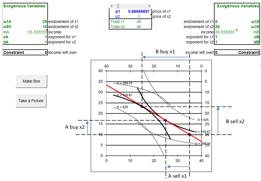
Figure 18.4: An Edgeworth Box in disequilibrium.

Source: EdgeworthBoxGE.xls!EdgeworthBox1.

We begin with A, which is easier than B. In Figure 18.4, arrows along the bottom and left sides of the box indicate what A wants to do: sell \(x_1\) and buy \(x_2\). It is natural to read the dashed lines from A’s optimal solution and see that left on the x axis means sell, while up on the y axis means buy.

Reading B is trickier. B also has arrows, but they run the reverse of the usual because we read B’s graph from the northeast corner. B wants to buy \(x_1\) and sell \(x_2\).

The direction of the arrow indicates buying or selling. Although one wants to buy and the other sell, the length of the arrows in Figure 18.4 show that the plans do not match. The length of the arrows indicate the amounts to be bought and sold. If the lengths are not equal, we are not in equilibrium.

We review the buy and sell decisions of B more carefully, to make sure there is no confusion. B wants to buy 20 units of good 1. From her initial endowment of 5 units, she wants to move left along the top axis, which means acquiring more \(x_1\), until she ends up with 25 units. On the other hand, she wants to sell \(13 \frac{1}{3}\) units of good 2, moving up the right axis which means she is reducing her desired amount of \(x_2\).

If you get in the habit of drawing dashed lines on an Edgeworth Box, either on a piece of paper or by inserting dashed line shapes in Excel or Word, from the optimal solution of A and B, you greatly increase your chances of reading the graph correctly. Those dashed lines are a visual cue that remind you to read A from the bottom left and B from the top right.

STEP Scroll down below the Edgeworth Box to see two supply and demand graphs.

These are the partial equilibrium markets for the two goods. Good 1 shows a shortage, with price below the intersection of supply and demand. Good 2 has demand and supply reversed from the usual display because the price on the y axis is \(p_1/p_2\). There is a surplus of \(x_2\) at \(p_1/p_2 = \frac{2}{3}\).

Both markets adjust simultaneously. We know there is upward pressure on \(p_1\) from the shortage and downward pressure on \(p_2\) from the surplus. This will make the price ratio rise and the price vector will become steeper.

STEP Use the scroll bar (over cells G15 and H15) to see how price changes affect the box. Set the price ratio to 1.5.

The spreadsheet does most of the hard work for you. A’s and B’s optimal solutions are instantly calculated. The market position cells immediately reflect the position of markets for each good at the new prices (where good 1 is one and a half times as expensive as good 2).

The Edgeworth Box is a live graph that reflects the new price vector. It shows that we have overshot the equilibrium price vector because we now have a surplus of good 1 and a shortage of good 2.

STEP Practice reading the Edgeworth Box. With \(\frac{p_1}{p_2} = 1.5\), use the graph to read the amounts that A and B want to buy and sell. Compute the surplus and shortage of each good from the box alone.

Verify (using the cells in the Market Position part of the sheet) that your answers are correct. Look at the graphs below the Edgeworth Box to make sure you understand that the Edgeworth Box conveys the same information about the position of each market.

STEP Play with the price vector, adjusting the scroll bar to set different price ratios and interpreting how the consumers will respond to each price ratio by using the Edgeworth Box.

As you rotate the price vector, you are the Walrasian auctioneer. You are calling out prices and the two consumers are reacting to them. The more you practice reading the Edgeworth Box, the more comfortable you will get with it.

As you adjust the price ratio, the price vector swings to and fro. It always rotates around the initial endowment (which would change if and only if any of the four initial endowment parameter values change). The tatonnement process is how the market responds to shortages and surpluses by changing prices in such a way that the surpluses and shortages are reduced, until they are completely eliminated.

There is, of course, no auctioneer in the real world, but price pressure from surpluses and shortages are quite real. Our model captures these pressures by the fiction of the auctioneer changing prices in response to disquilibrium in the two markets.

General Equilibrium

You have seen how shortages and surpluses push the price line to and fro, swinging around the initial endowment point.

We know that equilibrium means no tendency to change. We apply this definition of equilibrium to this particular model: when \(\frac{p_1}{p_2}\) has no tendency to change, we know we have settled to the equilibrium solution. The equilibrium solution generated by the market tells us how much \(x_1\) and \(x_2\) each consumer will end up with if the market is used and how much each consumer wants to buy and sell of each good.

STEP Use the scroll bar to find the equilibrium price vector.

The equilibrium solution in a General Equilibrium Pure Exchange Model is a canonical economics graph that is reproduced as Figure 18.5. If your screen does not look like this graph, set the price ratio to 1.

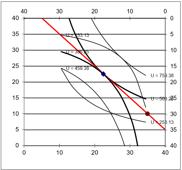
Figure 18.5: The canonical graph of general equilibrium.

Source: EdgeworthBoxGE.xls!EdgeworthBox1 with \(\frac{p_1}{p_2}=1\).

As Figure 18.5 clearly shows, when the equilibrium position is reached, the optimal solution of both consumers lies on the same point. This eliminates all shortages and surpluses (as shown in the supply and demand graphs below the Edgeworth Box) so the price ratio has no tendency to change.

The single point in the Edgeworth Box represents a mutually compatible solution for both consumers and is the hallmark of a general equilibrium solution. The single point is akin to the intersection of supply and demand in a partial equilibrium analysis.

Our general equilibrium model shows how the market is an allocation mechanism. It will redistribute the initial endowments of the two consumers by using prices until it settles down to a position where plans match and forces in the model are in balance.

Notice, however, that the two consumers don’t get equal amounts of the two goods. Why does A end up with more? Because A started out richer. At the equilibrium price vector, the market values A’s endowment at $45 and B’s at $35. General equilibrium theory does not ask why A is richer. It takes the initial endowment as given.

Walras’ Law

Leon Walras is the father of General Equilibrium Theory. The law that bears his name states the following: The value of aggregate excess demand is identically zero.

Using Walras’ Law, we can deduce the following logical result: If \(n–1\) markets are in equilibrium, then the last market must be in equilibrium.

A concrete demonstration of Walras’ Law is the best way to understand what it means.

STEP With \(p_1 = 1\) (at the equilibrium solution), change \(p_2\) (cell H17) to 2. Find the equilibrium \(p_1\).

The equilibrium \(p_1\) is now 2. This shows that, no matter the value of \(p_2\), the equilibrium solution will be found when \(\frac{p_1}{p_2}\) equals one.

Thus, it looks like there are two endogenous variables here, \(p_1\) and \(p_2\), but there is really only one endogenous variable, \(\frac{p_1}{p_2}\). This is the idea behind Walras’ Law and why we can find equilibrium in both markets by varying only \(p_1\).

STEP Click the button. Scroll right to cell V5 and click the button to reveal calculations that demonstrate Walras’ Law in action.

Although the two markets are not in equilibrium, the sum of the value of aggregate net demands in cell Y11 is zero. Look at the cell formulas in row 11 to see how they are computed.

STEP Change \(p_1\) (via the scroll bar) and notice that no matter the price, the sum of the value of aggregate net demand is always zero.

A direct implication of Walras’ Law is that in a general equilibrium system with n goods, we do not have to find n prices. If \(n - 1\) markets are in equilibrium, the last one automatically has to be in equilibrium.

This is why we actually have only a single endogenous variable, the price ratio, in the two-good case. All that matters is the relative price, not the two individual prices. With n goods, one good would be the numeraire (historically, gold has played that role) and all other goods would be valued in terms of the numeraire.

Comparative Statics with the Edgeworth Box

Having found the initial equilibrium solution, we could pursue a variety of comparative statics experiments, shocking an exogenous variable and tracking how the equilibrium solution (of various endogenous variables) responds.

STEP Click the button and then set cA (cell B21) to 2. What happened to A’s indifference curves and optimal solution?

With steeper indifference curves (since A likes good 1 more than before), A’s new tangency point is quite close to the initial endowment. This means A wants to sell little \(x_1\). You can scroll down to see how the partial equilibrium graphs have changedthe chart of \(x_1\) confirms we have a big shortage.

STEP Where is the new equilibrium solution? If you decide to use Solver to answer this question, please make the target cell H15 because that is the cell that the scroll bar is affecting. This way you will not destroy the formula in cell H16.

You should find a new equilibrium solution at a relative price ratio of about 1.53. Approximately 7.3 units of good 1 will be traded and 11.8 units of good 2 will be exchanged.

Two Advanced Ideas

In a mathematical sense, General Equilibrium Theory is perhaps the most abstract and sophisticated area of economics. Two questions that have been studied intensively involve existence and uniqueness.

The question of the existence of an equilibrium solution was posed by Walras himself. The issue, loosely stated, is that we cannot be sure that a general equilibrium system with thousands or millions of individual goods has a place where the entire system is at rest. In fact, from an intuitive point of view, given the huge number of products, consumers, and firms in a real-world economy, we might doubt that an equilibrium solution exists at all.

Walras and other early theorists thought that if the number of endogenous variables (unknowns) equaled the number of equations, then a solution was guaranteed. This is not so. Existence proofs in the 1950s utilized fixed-point theorems to prove rigorously the conditions under which an equilibrium solution was guaranteed to exist. Brouwer and Kakutani fixed point theorems are examples of this approach.

Closely tied to existence is the problem of the uniqueness of a general equilibrium solution. Even if an equilibrium solution is proved (in a rigorous mathematical sense) to exist, the worry is that there may be multiple equilibria in a general equilibrium system. Research has focused on what assumptions must be invoked to guarantee a single equilibrium solution.

Existence and uniqueness proofs are well beyond the scope of this book. They rely on topology and advanced mathematical concepts. This is another way of saying that our presentation of the Edgework Box and general equilibrium in a pure exchange economy is introductory and rudimentary. General Equilibrium Theory is a vast ocean and we are paddling near the shore.

Market Allocation in an Edgeworth Box

The canonical supply and demand graph is used in partial equilibrium analysis to find the equilibrium solution. General equilibrium uses the Edgeworth Box to do the same thing.

It appears cumbersome and tedious at first, but, in fact, it is an ingenious graphical device. By representing two consumers simultaneously, while sharing a common budget constraint (given that they face identical prices), the box enables one to quickly see whether the two-good, pure exchange economy is in equilibrium. It also reveals how prices must change as the system finds its way to equilibrium via the tatonnement process.

Whether a pure exchange economy is in a general equilibrium can be determined in an instant by seeing whether the optimal solutions of the two consumers are compatiblethat is, if there is a single point where the two consumers want to be, given the existing price ratio.

But what about the final, equilibrium allocation generated by the marketwhat are its properties? This is a fundamental question that leads to the famous Pareto optimality conditions and the First Fundamental Theorem of Welfare Economics. It is explained in the next section.

Although we have used numerical methods (implementing the problem in Excel) to analyze and find the general equilibrium solution, you should be aware that there are analytical approaches also. We could write down demands for goods by each consumer and impose the equilibrium condition that \(Q_D=Q_S\) in each market. This would enable solution of the equilibrium price vector with the aid of algebra (and, as soon as we left the simple world of two or three goods, linear algebra).

Exercises

1. Use Word’s Drawing Tools to draw your own Edgeworth Box. Place the initial endowment so that A has more \(x_2\) than \(x_1\).
2. Add a price vector to your box in the previous question that generates a shortage of \(x_1\). Draw arrows along the bottom and top \(x_1\) axes to show the amount of \(x_1\) each consumer wants to buy or sell.
3. Use Word’s Drawing Tools to draw a supply and demand graph for \(x_1\). Include a horizontal line in the graph that shows the current price of \(x_1\).
4. Add the equilibrium price vector to your Edgeworth Box graph in question 1. Explain why this price vector is the equilibrium solution.

   Hint: Add indifference curves to your graph to support your explanation.

References

The epigraph is from page 11 of Umberto Ricci, “Pareto and Pure Economics,” The Review of Economic Studies, Vol. 1, No. 1 (October, 1933), pp. 3–21, www.jstor.org/stable/2967433. You can learn more about Walras, Pareto, and the Lausanne School by visiting the History of Economic Thought web site at www.hetwebsite.net/het/.

Perhaps no area of economics is as mathematically sophisticated and intense as General Equilibrium Theory. There has always been disagreement among economists regarding the use and necessity of mathematics in economics. Pareto sneered at the literary economists and the use of math as a weapon continues today.

Akerlof says that economists only value "hard" and ignore "soft" questions so the discipline stifles research into issues that cannot be answered with formal tools and models. See George Akerlof (2020),"Sins of Omission and the Practice of Economics," doi.org/10.1257/jel.20191573, 58(2), 405–418, doi.org/10.1257/jel.20191573.

Roy Weintraub traces the influence of math in economics in How Economics Became a Mathematical Science, published in 2002. For the connection between economics and physics, see Phil Mirowski, More Heat than Light, published in 1989.