If long-run costs aren’t constant, how do changes in demand or costs affect short- and long-run prices and quantities traded?
The previous section made two simplifying assumptions that won’t hold in all applications of the theory. First, it assumed constant returns to scale, so that long-run supply is horizontal. A perfectly elastic long-run supply means that price always eventually returns to the same point. Second, the theory didn’t distinguish long-run from short-run demand. But with many products, consumers will adjust more over the long-term than immediately. As energy prices rise, consumers buy more energy-efficient cars and appliances, reducing demand. But this effect takes time to be seen, as we don’t immediately scrap our cars in response to a change in the price of gasoline. The short-run effect is to drive less in response to an increase in the price, while the long-run effect is to choose the appropriate car for the price of gasoline.
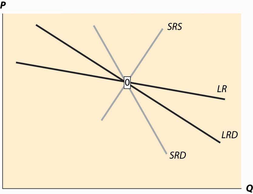
To illustrate the general analysis, we start with a long-run equilibrium. Figure 10.10 reflects a long-run economy of scale, because the long-run supply slopes downward, so that larger volumes imply lower cost. The system is in long-run equilibrium because the short-run supply and demand intersection occurs at the same price and quantity as the long-run supply and demand intersection. Both short-run supply and short-run demand are less elastic than their long-run counterparts, reflecting greater substitution possibilities in the long run.
Figure 10.10 Equilibrium with external scale economy
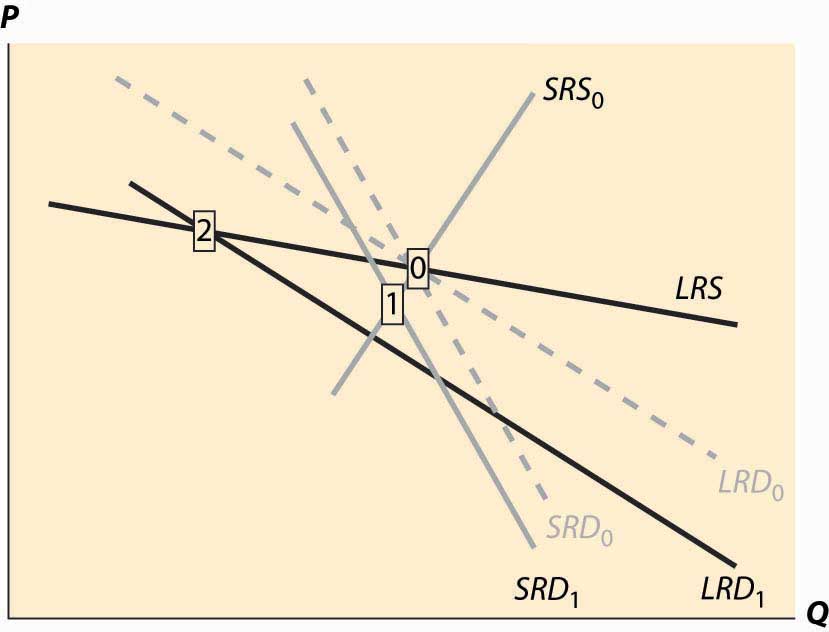
Figure 10.11 Decrease in demandFigure 10.11. To reduce the proliferation of curves, we colored the old demand curves very faintly and marked the initial long-run equilibrium with a zero inside a small rectangle.The short-run demand and long-run demand have been shifted down by the same amount; that is, both reflect an equal reduction in value. This kind of shift might arise if, for instance, a substitute had become cheaper; but the equal reduction is not essential to the theory. In addition, the fact of equal reductions often isn’t apparent from the diagram, because of the different slopes—to most observers, it appears that short-run demand fell less than long-run demand. This isn’t correct, however, and one can see this because the intersection of the new short-run demand and long-run demand occurs directly below the intersection of the old curves, implying both fell by equal amounts. The intersection of short-run supply and short-run demand is marked with the number 1. Both long-run supply and long-run demand are more elastic than their short-run counterparts, which has an interesting effect. The short-run demand tends to shift down over time, because the price associated with the short-run equilibrium is above the long-run demand price for the short-run equilibrium quantity. However, the price associated with the short-run equilibrium is below the long-run supply price at that quantity. The effect is that buyers see the price as too high, and are reducing their demand, while sellers see the price as too low, and so are reducing their supply. Both short-run supply and short-run demand fall, until a long-run equilibrium is achieved.
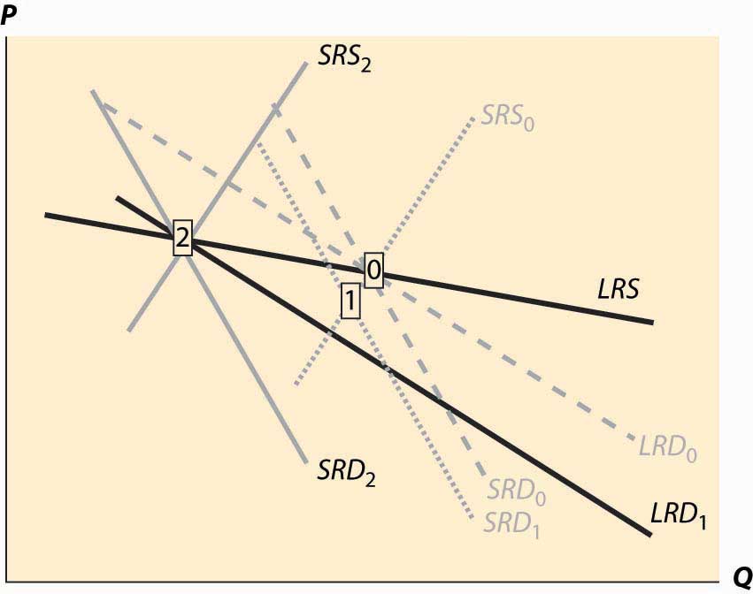
Figure 10.12 Long-run after a decrease in demand
Figure 10.12 illustrates. The new long-run equilibrium has short-run demand and supply curves associated with it, and the system is in long-run equilibrium because the short-run demand and supply, which determine the current state of the system, intersect at the same point as the long-run demand and supply, which determine where the system is heading.
There are four basic permutations of the dynamic analysis—demand increase or decrease and a supply increase or decrease. Generally, it is possible for long-run supply to slope down—this is the case of an economy of scale—and for long-run demand to slope up.The demand situation analogous to an economy of scale in supply is a network externality, in which the addition of more users of a product increases the value of the product. Telephones are a clear example—suppose you were the only person with a phone—but other products like computer operating systems and almost anything involving adoption of a standard represent examples of network externalities. When the slope of long-run demand is greater than the slope of long-run supply, the system will tend to be inefficient, because an increase in production produces higher average value and lower average cost. This usually means that there is another equilibrium at a greater level of production. This gives 16 variations of the basic analysis. In all 16 cases, the procedure is the same. Start with a long-run equilibrium and shift both the short-run and long-run levels of either demand or supply. The first stage is the intersection of the short-run curves. The system will then go to the intersection of the long-run curves.
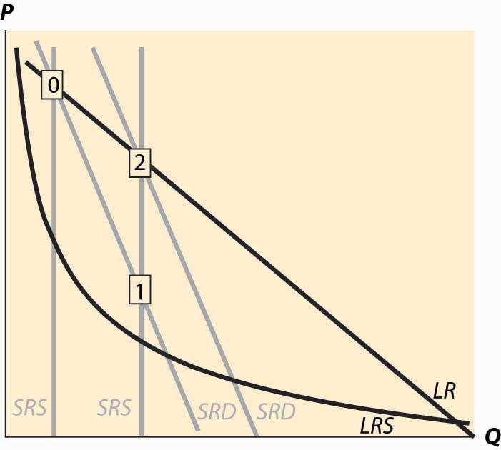
An interesting example of competitive dynamics’ concepts is the computer memory market, which was discussed previously. Most of the costs of manufacturing computer memory are fixed costs. The modern DRAM plant costs several billion dollars; the cost of other inputs—chemicals, energy, labor, silicon wafers—are modest in comparison. Consequently, the short-run supply is vertical until prices are very, very low; at any realistic price, it is optimal to run these plants 100% of the time.The plants are expensive, in part, because they are so clean—a single speck of dust falling on a chip ruins the chip. The Infineon DRAM plant in Virginia stopped operations only when a snowstorm prevented workers and materials from reaching the plant. The nature of the technology has allowed manufacturers to cut the costs of memory by about 30% per year over the past 40 years, demonstrating that there is a strong economy of scale in production. These two features—vertical short-run supply and strong economies of scale—are illustrated in Figure 10.13. The system is started at the point labeled with the number 0, with a relatively high price, and technology that has made costs lower than this price. Responding to the profitability of DRAM, short-run supply shifts out (new plants are built and die-shrinks permit increasing output from existing plants). The increased output causes prices to fall relatively dramatically because short-run demand is inelastic, and the system moves to the point labeled 1. The fall in profitability causes DRAM investment to slow, which allows demand to catch up, boosting prices to the point labeled 2. (One should probably think of Figure 10.13 as being in a logarithmic scale.)
Figure 10.13 DRAM market
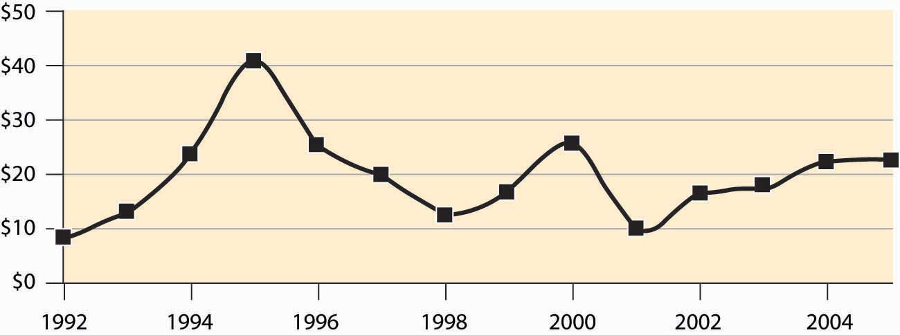
Figure 10.14, which shows DRAM industry revenues in billions of dollars from 1992 to 2003, and projections of 2004 and 2005.Two distinct data sources were used, which is why there are two entries for each of 1998 and 1999.
Figure 10.14 DRAM revenue cycle
KEY TAKEAWAY
In general, both demand and supply may have long-run and short-run curves. In this case, when something changes, initially the system moves to the intersections of the current short-run supply and demand for a short-run equilibrium, then to the intersection of the long-run supply and demand. The second change involves shifting short-run supply and demand curves.
EXERCISES
Land close to the center of a city is in fixed supply, but it can be used more intensively by using taller buildings. When the population of a city increases, illustrate the long- and short-run effects on the housing markets using a graph.
Emus can be raised on a wide variety of ranch land, so that there are constant returns to scale in the production of emus in the long run. In the short run, however, the population of emus is limited by the number of breeding pairs of emus, and the supply is essentially vertical. Illustrate the long- and short-run effects of an increase in demand for emus. (In the late 1980s, there was a speculative bubble in emus, with prices reaching $80,000 per breeding pair, in contrast to $2,000 or so today.)
There are long-run economies of scale in the manufacture of computers and their components. There was a shift in demand away from desktop computers and toward notebook computers around the year 2001. What are the short- and long-run effects? Illustrate your answer with two diagrams, one for the notebook market and one for the desktop market. Account for the fact that the two products are substitutes, so that if the price of notebook computers rises, some consumers shift to desktops. (To answer this question, start with a time 0 and a market in long-run equilibrium. Shift demand for notebooks out and demand for desktops in.) What happens in the short run? What happens in the long run to the prices of each? What does that price effect do to demand?