The analysis of behaviour necessarily involves data. Data may serve to validate or contradict a theory. Data analysis, even without being motivated by economic theory, frequently displays patterns of behaviour that merit examination. The terms variables and data are related. Variables are measures that can take on different magnitudes. The interest rate on a student loan, for example, is a variable with a certain value at a point in time but perhaps a different value at an earlier or later date. Economic theories and models explain the causal relationships between variables. In contrast, Data are the recorded values of variables. Sets of data provide specific values for the variables we want to study and analyze. Knowing that gross domestic product (a variable) declined in 2009 is just a partial description of events. If the data indicate that it decreased by exactly 3%, we know a great deal more – we know that the decline was significantly large.
Variables: measures that can take on different values.
Data: recorded values of variables.
Sets of data help us to test our models or theories, but first we need to pay attention to the economic logic involved in observations and modelling. For example, if sunspots or baggy pants were found to be correlated with economic expansion, would we consider these events a coincidence or a key to understanding economic growth? The observation is based on facts or data, but it need not have any economic content. The economist's task is to distinguish between coincidence and economic causation.
While the more frequent wearing of loose clothing in the past may have been associated with economic growth because they both occurred at the same time (correlation), one could not argue on a logical basis that this behaviour causes good economic times. Therefore, the past association of these variables should be considered as no more than a coincidence. Once specified on the basis of economic logic, a model must be tested to determine its usefulness in explaining observed economic events.
Table 2.1 House prices and price indexes
| Year |
House |
Percentage |
Percentage |
Real |
Index for |
5-year |
| |
prices in |
change in  |
change in |
percentage |
price of |
mortgage |
| |
dollars |
|
consumer |
change |
housing |
rate |
| |
( ) ) |
|
prices |
in  |
|
|
| 2001 |
350,000 |
|
|
|
100 |
7.75 |
| 2002 |
360,000 |
|
|
|
102.9 |
6.85 |
| 2003 |
395,000 |
35,000/360,000=9.7% |
3% |
6.7% |
112.9 |
6.6 |
| 2004 |
434,000 |
|
|
|
124.0 |
5.8 |
| 2005 |
477,000 |
|
|
|
136.3 |
6.1 |
| 2006 |
580,000 |
|
|
|
165.7 |
6.3 |
| 2007 |
630,000 |
|
|
|
180.0 |
6.65 |
| 2008 |
710,000 |
|
|
|
202.9 |
7.3 |
| 2009 |
605,000 |
-105,000/710,000=-14.8% |
1.6% |
-16.4% |
172.9 |
5.8 |
| 2010 |
740,000 |
|
|
|
211.4 |
5.4 |
| 2011 |
800,000 |
|
|
|
228.6 |
5.2 |
Note: Data on changes in consumer prices come from Statistics Canada, CANSIM series V41692930; data on house prices are for N. Vancouver from
Royal Le Page; data on mortgage rates from
www.ratehub.ca. Index for house prices obtained by scaling each entry in column 2 by 100/350,000. The real percentage change in the price of housing is: The percentage change in the price of housing minus the percentage change in consumer prices.
Data types
Data come in several forms. One form is time-series, which reflects a set of measurements made in sequence at different points in time. The first column in Table 2.1 reports the values for house prices in North Vancouver for the first quarter of each year, between 2001 and 2011. Evidently this is a time series. Annual data report one observation per year. We could, alternatively, have presented the data in monthly, weekly, or even daily form. The frequency we use depends on the purpose: If we are interested in the longer-term trend in house prices, then the annual form suffices. In contrast, financial economists, who study the behaviour of stock prices, might not be content with daily or even hourly prices; they may need prices minute-by-minute. Such data are called high-frequency data, whereas annual data are low-frequency data.
Table 2.2 Unemployment rates, Canada and Provinces, monthly 2012, seasonally adjusted
| |
Jan |
Feb |
Mar |
Apr |
May |
Jun |
| CANADA |
7.6 |
7.4 |
7.2 |
7.3 |
7.3 |
7.2 |
| NFLD |
13.5 |
12.9 |
13.0 |
12.3 |
12.0 |
13.0 |
| PEI |
12.2 |
10.5 |
11.3 |
11.0 |
11.3 |
11.3 |
| NS |
8.4 |
8.2 |
8.3 |
9.0 |
9.2 |
9.6 |
| NB |
9.5 |
10.1 |
12.2 |
9.8 |
9.4 |
9.5 |
| QUE |
8.4 |
8.4 |
7.9 |
8.0 |
7.8 |
7.7 |
| ONT |
8.1 |
7.6 |
7.4 |
7.8 |
7.8 |
7.8 |
| MAN |
5.4 |
5.6 |
5.3 |
5.3 |
5.1 |
5.2 |
| SASK |
5.0 |
5.0 |
4.8 |
4.9 |
4.5 |
4.9 |
| ALTA |
4.9 |
5.0 |
5.3 |
4.9 |
4.5 |
4.6 |
| BC |
6.9 |
6.9 |
7.0 |
6.2 |
7.4 |
6.6 |
Source: Statistics Canada CANSIM Table 282-0087.
Time-series: a set of measurements made sequentially at different points in time.
High (low) frequency data: series with short (long) intervals between observations.
In contrast to time-series data, cross-section data record the values of different variables at a point in time. Table 2.2 contains a cross-section of unemployment rates for Canada and Canadian provinces economies. For January 2012 we have a snapshot of the provincial economies at that point in time, likewise for the months until June. This table therefore contains repeated cross-sections.
When the unit of observation is the same over time such repeated cross sections are called longitudinal data. For example, a health survey that followed and interviewed the same individuals over time would yield longitudinal data. If the individuals differ each time the survey is conducted, the data are repeated cross sections. Longitudinal data therefore follow the same units of observation through time.
Cross-section data: values for different variables recorded at a point in time.
Repeated cross-section data: cross-section data recorded at regular or irregular intervals.
Longitudinal data: follow the same units of observation through time.
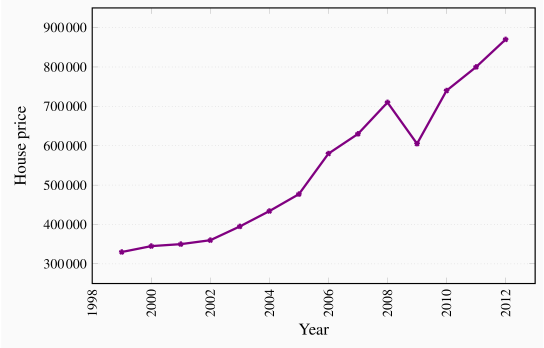
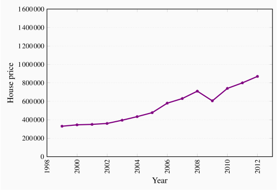
Graphing the data
Data can be presented in graphical as well as tabular form. Figure 2.1 plots the house price data from the second column of Table 2.1. Each asterisk in the figure represents a price value and a corresponding time period. The horizontal axis reflects time, the vertical axis price in dollars. The graphical presentation of data simply provides a visual rather than numeric perspective. It is immediately evident that house prices increased consistently during this 11-year period, with a single downward 'correction' in 2009. We have plotted the data a second time in Figure 2.2 to illustrate the need to read graphs carefully. The greater apparent slope in Figure 2.1 might easily be interpreted to mean that prices increased more steeply than suggested in Figure 2.2. But a careful reading of the axes reveals that this is not so; using different scales when plotting data or constructing diagrams can mislead the unaware viewer.
Percentage changes
The use of percentages makes the analysis of data particularly simple. Suppose we wanted to compare the prices of New York luxury condominiums with the prices of homes in rural Mississippi. In the latter case, a change in average prices of $10,000 might be considered enormous, whereas a change of one million dollars in New York might be pretty normal – because the average price in New York is so much higher than in Mississippi. To make comparisons between the two markets, we can use the concept of a percentage change. This is defined as the change in the value of the variable, relative to its initial value, multiplied by 100.
 .
.
The third column of Table 2.1 contains the values of the percentage change in house prices for two pairs of years. Between 2002 and 2003 the price change was $35,000. Relative to the price in the first of these two years this change was the fraction 35,000/395,000=0.097. If we multiply this fraction by 100 we obtain a percentage price change of 9.7%. Evidently we could calculate the percentage price changes for all pairs of years. A second price change is calculated for the 2008-2009 pair of years. Here price declined and the result is thus a negative percentage change.
Consumer prices
Most variables in economics are averages of the components that go into them. When variables are denominated in dollar terms it is important to be able to interpret them correctly. While the house price series above indicates a strong pattern of price increases, it is vital to know if the price of housing increased more or less rapidly that other prices in the economy. If all prices in the economy were increasing in line with house prices there would be no special information in the house price series. However, if house prices increased more rapidly than prices in general, then the data indicate that something special took place in the housing market during the decade in question. To determine an answer to this we need to know the degree to which the general price level changed each year.
Statistics Canada regularly surveys the price of virtually every product produced in the economy. One such survey records the prices of goods and services purchased by consumers. Statistics Canada then computes an average price level for all of these goods combined for each time period the survey is carried out (monthly). Once Statistics Canada has computed the average consumer price, it can compute the change in the price level from one period to the next. In Table 2.1 two such values are entered in the following data column: Consumer prices increased by 3% between 2002 and 2003, and by 1.6% between 2008 and 2009. These percentage changes in the general price level represent inflation if prices increase, and deflation if prices decline.
In this market it is clear that housing price changes were substantially larger than the changes in consumer prices for these two pairs of years. The next column provides information on the difference between the house price changes and changes in the general consumer price level, in percentage terms. This is (approximately) the change in the relative price of housing, or what economists call the real price of housing.
Consumer price index: the average price level for consumer goods and services.
Inflation (deflation) rate: the annual percentage increase (decrease) in the level of consumer prices.
Real price: the actual price adjusted by the general (consumer) price level in the economy.
Index numbers
Statistics Canada and other statistical agencies frequently present data in index number form. An index number provides an easy way to read the data. For example, suppose we wanted to compute the percentage change in the price of housing between 2001 and 2007. We could do this by entering the two data points in a spreadsheet or calculator and do the computation. But suppose the prices were entered in another form. In particular, by dividing each price value by the first year value and multipling the result by 100 we obtain a series of prices that are all relative to the initial year – which we call the base year. The resulting series in column 6 is an index of house price values. Each entry is the corresponding value in column 2, divided by the first entry in column 2. The key characteristics of indexes are that they are not dependent upon the units of measurement of the data in question, and they are interpretable easily with reference to a given base value. To illustrate, suppose we wish to know how prices behaved between 2001 and 2007. The index number column immediately tells us that prices increased by 80%, because relative to 2001, the 2007 value is 80% higher.
Index number: value for a variable, or an average of a set of variables, expressed relative to a given base value.
Furthermore, index numbers enable us to make comparisons with the price patterns for other goods much more easily. If we had constructed a price index for automobiles, which also had a base value of 100 in 2001, we could make immediate comparisons without having to compare one set of numbers defined in thousands of dollars with another defined in hundreds of thousands of dollars. In short, index numbers simplify the interpretation of data.