5.4: Business cycles and output gaps

Last updated
Save as PDF

Page ID: 45757

$ \newcommand{\vecs}[1]{\overset { \scriptstyle \rightharpoonup} {\mathbf{#1}} } $ $ \newcommand{\vecd}[1]{\overset{-\!-\!\rightharpoonup}{\vphantom{a}\smash {#1}}} $$\newcommand{\id}{\mathrm{id}}$ $ \newcommand{\Span}{\mathrm{span}}$ $ \newcommand{\kernel}{\mathrm{null}\,}$ $ \newcommand{\range}{\mathrm{range}\,}$ $ \newcommand{\RealPart}{\mathrm{Re}}$ $ \newcommand{\ImaginaryPart}{\mathrm{Im}}$ $ \newcommand{\Argument}{\mathrm{Arg}}$ $ \newcommand{\norm}[1]{\| #1 \|}$ $ \newcommand{\inner}[2]{\langle #1, #2 \rangle}$ $ \newcommand{\Span}{\mathrm{span}}$ $\newcommand{\id}{\mathrm{id}}$ $ \newcommand{\Span}{\mathrm{span}}$ $ \newcommand{\kernel}{\mathrm{null}\,}$ $ \newcommand{\range}{\mathrm{range}\,}$ $ \newcommand{\RealPart}{\mathrm{Re}}$ $ \newcommand{\ImaginaryPart}{\mathrm{Im}}$ $ \newcommand{\Argument}{\mathrm{Arg}}$ $ \newcommand{\norm}[1]{\| #1 \|}$ $ \newcommand{\inner}[2]{\langle #1, #2 \rangle}$ $ \newcommand{\Span}{\mathrm{span}}$$\newcommand{\AA}{\unicode[.8,0]{x212B}}$

In some years GDP grows very rapidly, and in other years it actually falls. Growth of potential GDP is also variable but it is consistently positive. These up and down fluctuations in the growth of real GDP are described as business cycles in economic activity.

Business cycles: short-term fluctuations of actual real GDP.

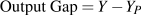
Business cycles cause differences between actual and potential GDP. Output gaps measure these differences. In a short-run aggregate demand and supply model with a constant potential output, the gap is:

(5.1)

Output gap: the difference between actual output and potential output.

In an economy that grows over time the absolute output gap Y–Y_P is usually measured relative to potential output. This recognizes that a gap of $10 million is a more serious matter in an economy with a potential output of $1,000 million than in an economy with a potential output of $5,000 million.

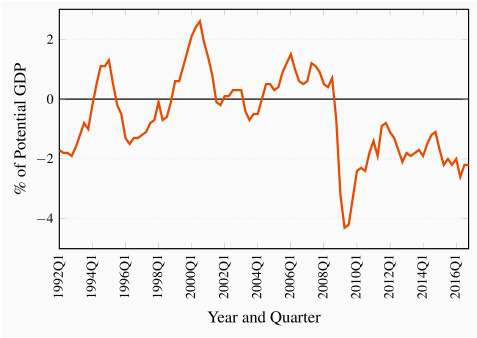
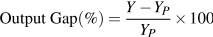
Figure 5.6 plots the Bank of Canada's estimates of the differences between actual and potential GDP for Canada for each year from 1992Q1 to 2016Q4, expressed as a percentage of potential GDP, calculated as:

(5.2)

Figure 5.6 The Output Gap in Canada, 1992Q1–2016Q4

Source: Bank of Canada, Indicators of Capacity and Inflation Pressures for Canada, www.bankofcanada.ca.

When we compare growth in actual real GDP and potential GDP in Canada from 2007 to 2013 in Figure 5.5, we see an example of the business cycle caused by the 2008 – 2009 financial crisis. Real GDP growth declined in 2008 to less than growth potential GDP and turned negative in 2009. This was a recession. It created the negative output gap in Figure 5.6 that starts in the first quarter of 2009 and persists in the most recent data for the fourth quarter of 2016.

Output gaps describe and measure the short-run economic conditions, and indicate the strength or weakness of the economy's performance. High growth rates in the boom phase of the cycle create positive output gaps, which are called inflationary gaps because they put upward pressure on costs and prices. Low or negative growth rates that result in negative output gaps and rising unemployment rate are called recessionary gaps. They put downward pressure on costs and prices. As economic conditions change over time, business cycle fluctuations move the economy through recessionary and inflationary gaps. However, you will notice in Figure 5.6 that recessionary gaps in Canada have been deeper and more persistent than inflationary gaps over the past 30 years.

Inflationary gap: a measure of the amount by which actual GDP is greater than potential GDP.

Recessionary gap: a measure of the amount by which actual GDP is less than potential GDP.

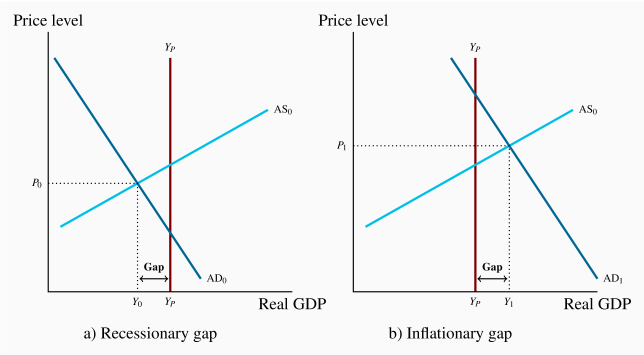
We can show output gaps in diagrams using the aggregate demand and supply curves and the potential output line introduced in Figures 5.1 and 5.4. Figure 5.7 provides an example. Panel a) illustrates a recessionary gap. Panel b) shows an inflationary gap.

Figure 5.7 Output Gap

In Figure 5.7 panel a) shows a recessionary gap because AD is too weak to support equilibrium at Y_P. Alternatively in panel b) AD is too strong and pushes equilibrium past Y_P.

The AD and AS model provides a basic explanation of the differences we see between actual real GDP and potential real GDP. Short-run AD and AS conditions determine equilibrium real GDP, which may be either greater or less than potential GDP. Furthermore, the business cycles are the results of changes in the short-run AD and AS conditions.

Introduction to the AD/AS model is an important first step in the study of the performance of the macro economy. But there are more questions:

What is the relationship between output gaps and unemployment?
How would the economy react to a persistent output gap?
Why do short-run AD and AS conditions change from time to time?

The first two questions are considered in the remainder of this chapter. Chapter 6 starts on the third question.