National Accounts as in Chapter 4 measure actual expenditure, output and national income and GDP(Y). The Aggregate Expenditure function gives planned expenditure (AE). In a modern industrial economy actual output and income may differ from what was planned, either on the output side or on the purchase and sales side. A simple example of the time sequence of output and sales shows why.
In most cases business install capacity and produce output in anticipation of sales in the near future. This is apparent from the stocks of goods offered in most retail outlets or online. Auto manufacturers, for example like to have an inventory of 30 to 60 days of finished vehicle sales available for retail buyers. Coffee and donut shops have coffee and snacks available to customers when they walk in. Even service industries like cell phone companies try to have staff and product on hand and ready to serve customers on demand. In these and other cases producers incur costs that they expect to recover from later sales. If sales don't match expectations some inventories of products build up or fall short, capacity is not matched to demand and some sales opportunities are lost or costs are not recovered.
As a result, if planned expenditure (AE) and GDP are different then plans in some part of the economy have not been realized and there is an incentive to change output. However, when actual output (GDP) is equal to planned expenditure (AE) expenditure and output plans are successful and, unless underlying conditions change there is no incentive to change output.
Equilibrium output
Output is said to be in short-run equilibrium when the current output of goods and services equals planned aggregate expenditure:
Y=A0+(c–m)Y
(6.2)
Then spending plans are not frustrated by a shortage of goods and services. Nor do business firms make more output than they can sell. In short-run equilibrium, output equals the total of goods and services households, businesses, and residents of other countries want to buy. Real GDP is determined by aggregate expenditure.
Short-run equilibrium output: Aggregate expenditure and current output are equal ().
Figure 6.7 The diagram and equilibrium GDP
The line gives the equilibrium condition. At point E the AE line crosses the line and . This is the equilibrium. At Y1, AE>Y and unplanned reductions in inventories provide the incentive to increase Y.
line labeled , illustrates the equilibrium condition. At every point on the line, AE measured on the vertical axis equals current output, Y, measured on the horizontal axis. This line has a slope of 1.Figure 6.7 starts from a positive intercept on the vertical axis to show autonomous aggregate expenditure A0, and has a slope equal to (c–m) which is less than one. The line has a slope equal to one. At every point on the line, the value of output (and income) measured on the horizontal axis equals the value of expenditure on the vertical axis. With a positive vertical intercept and slope less than 1 the AE line crosses the line at E. Since E is the only point on the AE line also on the line, it is the only point at which output and planned expenditure are equal. It is the equilibrium point.
Income Y2 is the only income at which aggregate expenditure just buys all current output. For example, assume as shown in the diagram, that output and incomes are only Y1. Aggregate expenditure at D is not equal to output as measured at B. Planned expenditure is greater than current output. Aggregate spending plans cannot all be fulfilled at this current output level. Consumption and export plans will be realized only if business fails to meet its investment plans as a result of an unplanned fall in inventories of goods.
In Figure 6.7 all outputs less than the equilibrium output Y2, are too low to satisfy planned aggregate expenditure. The AE line is above the line along which expenditure and output are equal. Conversely, if real GDP is greater than Y2 aggregate expenditure is not high enough to buy all current output produced. Businesses have unwanted and unplanned increases in inventories of unsold goods.
Table 6.3 extends the numerical example in Table 6.2 to show equilibrium when GDP(Y) is 200 and the unwanted inventory changes at other income levels. When GDP in column (1) is less than AE in column (4) current output does not cover current planned expenditure. Inventories fall and producers can't meet their inventory targets. The unwanted change in inventories in column (5) is negative.
Table 6.3 Equilibrium GDP: .
GDP (Y)
Autonomous
Induced
Aggregate
Unplanned
Expenditure
Expenditure
Expenditure
Inventory
(A0=100)
(c–m)Y=0.5Y
(1)
(2)
(3)
(4)
(5)
0
100
0
100
-100
50
100
25
125
-75
100
100
50
150
-50
175
100
87.5
187.5
-12.5
200
100
100
200
0
250
100
125
225
+25
300
100
150
250
+50
You can construct a diagram like Figure 6.7 using the numerical values for GDP and aggregate expenditure in Table 6.3 and a line to show equilibrium Ye=200. Example Box 6.1 at the end of the chapter illustrates equilibrium for this basic model using simple algebra.
Adjustment towards equilibrium
Unplanned changes in business inventories cause adjustments in output that move the economy to equilibrium output. Suppose in Figure 6.7 the economy begins with an output Y1, below equilibrium output Ye. Aggregate expenditure is greater than output Y1. If firms have inventories from previous production, they can sell more than they have produced by running down inventories for a while. Note that this fall in inventories is unplanned. Planned changes in inventories are already included in planned investment and aggregate expenditure.
Unplanned changes in business inventories: indicators of disequilibrium between planned and actual expenditures – incentives for businesses to adjust levels of employment and output (Y).
If firms cannot meet planned aggregate expenditure by unplanned inventory reductions, they must turn away customers. Either response—unplanned inventory reductions or turning away customers—is a signal to firms that aggregate expenditure is greater than current output, markets are strong, and output and sales can be increased profitably. Hence, at any output below Ye, aggregate expenditure exceeds output and firms get signals from unwanted inventory reductions to raise output.
Conversely, if output is initially above the equilibrium level, Figure 6.7 shows that output will exceed aggregate expenditure. Producers cannot sell all their current output. Unplanned and unwanted additions to inventories result, and firms respond by cutting output. In the last few years, producers of commodities including iron ore, copper, metallurgical coal, base metals, natural gas, and crude oil have faced declining demand for their products and lower prices and rising inventories. Producers responded by lowering production to try to reduce excess inventory. In general terms, when the economy is producing more than current aggregate expenditure, unwanted inventories build up and output is cut back.
Hence, when output is below the equilibrium level, firms raise output. When output is above the equilibrium level, firms reduce output. At the equilibrium output Ye, firms sell their current output and there are no unplanned changes to their inventories. Firms have no incentive to change output.
Equilibrium output and employment
In the examples of short-run equilibrium we have discussed, output is at Ye with output equal to planned expenditure. Firms sell all they produce, and households and firms buy all they plan to buy. But it is important to note that nothing guarantees that equilibrium output Ye is the level of potential output YP. When wages and prices are fixed, the economy can end up at a short-run equilibrium below potential output with no forces present to move output to potential output. Furthermore, we know that, when output is below potential output, employment is less than full and the unemployment rate u is higher than the natural rate un. The economy is in recession and by our current assumptions neither price flexibility nor government policy action can affect these conditions.


 ).
). diagram and equilibrium GDP
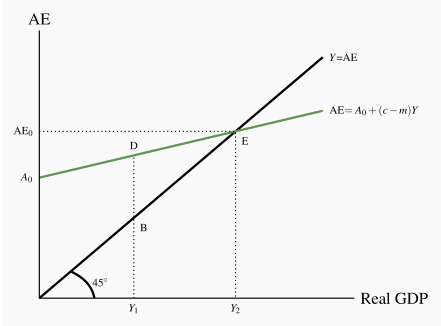
 line gives
  the equilibrium condition. At point E the AE line crosses the
  line and
  . This is the equilibrium. At Y1, AE>Y and unplanned reductions in inventories provide the incentive to increase Y.
 line labeled
  , illustrates the equilibrium condition. At every point on the
  line, AE measured on the vertical axis equals current output, Y, measured on the horizontal axis. This
  line has a slope of 1.
 line has a slope equal to one. At every point on the
  line, the value of output (and income) measured on the horizontal axis equals the value of expenditure on the vertical axis. With a positive vertical intercept and slope less than 1 the AE line crosses the
  line at E. Since E is the only point on the AE line also on the
  line, it is the only point at which output and planned expenditure are equal. It is the equilibrium point.
 line along which expenditure and output are equal. Conversely, if real GDP is greater than Y2 aggregate expenditure is not high enough to buy all current output produced. Businesses have unwanted and unplanned increases in inventories of unsold goods.
 .
. Inventory

 line to show equilibrium Ye=200. Example Box 6.1 at the end of the chapter illustrates equilibrium for this basic model using simple algebra.