6.4: The multiplier - Changes in aggregate expenditure and equilibrium output
- Page ID
- 45766

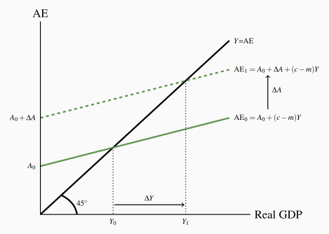
Suppose firms become very optimistic about future demand for their output. They want to expand their factories and add new equipment to meet this future demand. Autonomous expenditure rises. If other components of aggregate expenditure are unaffected, AE will be higher at each income than before. Figure 6.8 shows this upward shift in AE to  . Before we go into detail, think about what is likely to happen to output. It will rise, but by how much?
 shifts AE up to
  . Equilibrium GDP rises by a larger amount from Y0 to Y1.
 ). Firms increase output again to meet this increased demand, further increasing household incomes. Consumption and imports rise further. This is a first and important example of interdependency and feedback in a basic model. A change in autonomous expenditure, either positive or negative, changes income which in turn causes a change in induced expenditure. Equilibrium income changes by the change in autonomous expenditure plus the change in induced expenditure.
 line. Households increase their expenditure when incomes rise, but they increase expenditure by less than the rise in income. Equilibrium moves from Y0 to Y1. Equilibrium output rises more than the original rise in investment,
  , but does not rise without limit.
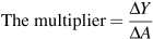 |
(6.3) |
Multiplier  : the ratio of the change in equilibrium income Y to the change in autonomous expenditure A that caused it.
| Initial | New | Initial | New | ||
| GDP | Autonomous | Autonomous | Induced | Aggregate | Aggregate |
| (Y) | Expenditure | Expenditure | Expenditure | Expenditure | Expenditure |
| (A0=100) | (A1=125) | (c–m)Y=0.5Y |  |
 |
|
| (1) | (2) | (3) | (4) | (5) | (6) |
| 175 | 100 | - | 87.5 | 187.5 | 187.5 |
| 200 | 100 | - | 100 | 200 | 200 |
| 225 | 125 | 112.5 | 237.5 | ||
| 237.5 | 125 | 118.75 | 243.5 | ||
| 243.5 | 125 | 121.75 | 246.75 | ||
| 246.75 | 125 | ||||
| – | 125 | ||||
| 250 | 125 | 125 | 250 | ||
| 300 | 125 | 150 | 275 |
The initial increase in aggregate expenditure illustrated is from 200 to 237.5 made up of an increase in autonomous expenditure of 25 and in induced expenditure of  . However GDP(Y) is only 225 and planned expenditure is accommodated by a decrease in inventories of 12.5. This unintended fall in inventories is an incentive to increase production to take advantage of higher than expected sales. The incentive exists until producers increase output and income to 250. Aggregate expenditure rises as income increases until equilibrium is reached at Y=250. At that point actual inventory investment meets producer plans.
 .
. line to show equilibrium Ye=200. Example Box 6.2 at the end of the chapter illustrates the multiplier effect of a change in autonomous expenditure on equilibrium income using simple algebra.
The size of the multiplier
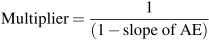 |
(6.4) |
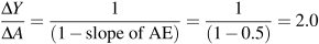
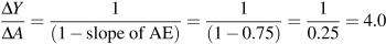
But at a different time or in a different economy the marginal propensity to consume might be higher and the marginal propensity to import might be lower, for example let c1=0.85 and m1=0.10. Then induced expenditure on domestic output would be (c1–m1)=(0.85–0.10)=0.75 as would the slope of  . Now a change in autonomous expenditure raises income and causes a higher change in induced expenditure. As a result the multiplier for this economy would be: