
7.7: Aggregate demand and equilibrium output
- Page ID
- 45776

\( \newcommand{\vecs}[1]{\overset { \scriptstyle \rightharpoonup} {\mathbf{#1}} } \) \( \newcommand{\vecd}[1]{\overset{-\!-\!\rightharpoonup}{\vphantom{a}\smash {#1}}} \)\(\newcommand{\id}{\mathrm{id}}\) \( \newcommand{\Span}{\mathrm{span}}\) \( \newcommand{\kernel}{\mathrm{null}\,}\) \( \newcommand{\range}{\mathrm{range}\,}\) \( \newcommand{\RealPart}{\mathrm{Re}}\) \( \newcommand{\ImaginaryPart}{\mathrm{Im}}\) \( \newcommand{\Argument}{\mathrm{Arg}}\) \( \newcommand{\norm}[1]{\| #1 \|}\) \( \newcommand{\inner}[2]{\langle #1, #2 \rangle}\) \( \newcommand{\Span}{\mathrm{span}}\) \(\newcommand{\id}{\mathrm{id}}\) \( \newcommand{\Span}{\mathrm{span}}\) \( \newcommand{\kernel}{\mathrm{null}\,}\) \( \newcommand{\range}{\mathrm{range}\,}\) \( \newcommand{\RealPart}{\mathrm{Re}}\) \( \newcommand{\ImaginaryPart}{\mathrm{Im}}\) \( \newcommand{\Argument}{\mathrm{Arg}}\) \( \newcommand{\norm}[1]{\| #1 \|}\) \( \newcommand{\inner}[2]{\langle #1, #2 \rangle}\) \( \newcommand{\Span}{\mathrm{span}}\)\(\newcommand{\AA}{\unicode[.8,0]{x212B}}\)
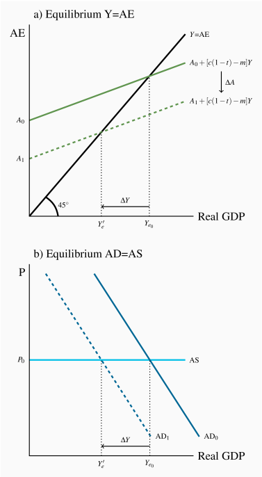
Figure 7.11 shows the relationship between equilibrium income and output, and the link between changes in aggregate expenditure, aggregate demand, and equilibrium income. In the upper diagram a fall in autonomous expenditure from A0 to A1 reduces AE and equilibrium Y from  to
to  , which is the fall in A times the multiplier.
Figure 7.11 AE, AD and equilibrium output
Example Box 7.1 The effect of the government sector on equilibrium income
| a) Equilibrium with no Government | |||
| Autonomous expenditure | =A0 | Autonomous expenditure | =80 |
| Induced expenditure | =(c–m)Y | Induced expenditure | =(0.8–0.2)Y=0.6Y |
| Aggregate expenditure | =A0+(c–m)Y | Aggregate expenditure | =80+0.6Y |
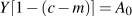
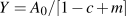
| Equilibrium income: |  |
Equilibrium income: |  |
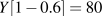
| Y=A0+(c–m)Y | Y=80+0.6Y | ||
 |
 |
||
 |
 |
||
| Y=200 | |||
|
|
|||
| b) Equilibrium with added government sector: G=25, NT=0.10Y | |||
| Autonomous expenditure | =A0+G0 | Autonomous expenditure | =105 |
| Induced expenditure | =c(1–t)–m | Induced expenditure |  |
| Aggregate expenditure |  |
Aggregate expenditure | =105+0.52Y |
| Equilibrium income: |  |
Equilibrium income: |  |
 |
Y=105+0.52Y | ||
 |
Y(1–0.52)=105 | ||
 |
 |
||
| Y=218.4 | |||
In this example adding government expenditure G=25 financed in part by a net tax rate t=0.10 raised autonomous expenditure by 25 but lowered the multiplier from 2.5 to 2.08 with the result that equilibrium income increased by 18.4. Equilibrium income increased because the government sector ran a budget deficit. G was 25 but net tax revenue was only  .
.