9.5: Interest rates, exchange rates, and aggregate demand

Interest rates and exchange rates link the changes in money and financial markets to the expenditure decisions that determine aggregate demand.

The impact of financial markets, interest rates, and exchange rates on aggregate expenditure, aggregate demand, and real output is described by the transmission mechanism. It has three important channels, namely:

1. the effect of interest rate changes on consumption expenditure;
2. the effect of interest rate changes on investment expenditure; and
3. the effect of interest rate changes on foreign exchange rates and net exports.

Transmission mechanism: links money, interest rates, and exchange rates through financial markets to output and employment and prices.

Interest rates and consumption expenditure

The basic consumption function in Chapter 6 was illustrated by a straight line relating aggregate consumption to disposable income. The positive slope of that line, the marginal propensity to consume, showed the change in consumption expenditure that would result from a change in disposable income. The vertical intercept of the consumption function showed autonomous consumption expenditure, the consumption expenditure not determined by disposable income. Changes in income moved households along the consumption function. Changes in autonomous consumption expenditure changed the vertical intercept, shifting the consumption function up or down.

Changes in interest rates affect autonomous consumption expenditure in two ways.

1. Through a wealth effect from changes in the prices of financial assets; and
2. Through a cost of credit effect.

Wealth effect: the change in expenditure caused by a change in real wealth.

Cost of credit: the cost of financing expenditures by borrowing at market interest rates.

The market prices of bonds are the present values of expected future interest and principal payments. Current market interest rates are the key factor in this relationship. Similarly, interest rates and the expected stream of profits and dividend payments determine the present values and prices of company shares. Lower discount rates give higher present values and higher interest rates reduce present values. As a result, falling interest rates raise financial asset prices and rising interest rates reduce financial asset prices.

This means that changes in interest rates, by changing prices of financial assets, change the wealth held in household portfolios. A fall in market interest rates raises household financial wealth which increases household consumption expenditure. Autonomous consumption expenditure increases as a result of this wealth effect. A rise in interest rates would reduce autonomous consumption expenditure.

Changes in interest rates also have important effects on house prices by lowering the cost of credit, increasing the present values of rental incomes, and increasing the market prices of residential real estate. Households often used the increased market values and equity in their housing to set up home equity lines of credit with relatively low borrowing rates. This borrowing is used to finance other expenditures. Autonomous consumption expenditures change as interest rate changes change the cost and extent of this financing.

Thus, two forces—wealth effects, and availability and cost of credit—explain the effects of money on planned consumption expenditure. This is one part of the transmission mechanism through which money and interest rates affect expenditure. Operating through wealth effects and the supply and cost of credit, changes in money supply and interest rates shift the consumption function. We can recognize the effects of both income and interest rates on consumption by using an equation, namely:

Consumption expenditure depends on both national income and interest rates, or:

(9.2)

The marginal propensity to consume out of national income is a positive fraction, , and the relationship between consumption and interest rates is negative, .

When consumption expenditure is plotted relative to national income as in the line diagrams of Chapters 6 and 7, a change in the interest rate shifts the consumption function but does not change its slope.

Interest rates and investment expenditure

In Chapters 4 and 6 we defined investment expenditure as the purchase of currently produced fixed capital, which includes plants, machinery and equipment; and inventories of raw materials, components, and finished goods. Spending on new residential and non-residential construction is also included in investment. Assume investment is independent of current income and therefore an autonomous component of aggregate expenditure. However, the interest rates determined in money and financial markets affect investment expenditure.

The data in Chapters 4 and 6 showed investment at about 20 percent of GDP in 2016 but with the level of investment spending changing from year to year within a range of +/- 11 percent. Although the total change in inventories is quite small, this component of total investment is volatile and contributes to the fluctuations in the total level of investment. Interest rate changes are responsible for some part of the volatility in investment spending.

Government capital expenditures on buildings, roads, bridges, and machinery and equipment are a part of government expenditure G. We treat government capital expenditure as part of fiscal policy and include it in G, not in I.

Businesses spend on fixed capital, plant and equipment to expand their output capacity if they expect growth in demand for their output, or if they see opportunities to reduce costs by adopting new technology and production techniques. Wireless companies like Bell Canada, Rogers and Telus spend continuously on new equipment to accommodate subscriber growth and new products that require more and faster data and voice transmission. Auto makers add to or reduce assembly capacity and develop new product and production technologies to remain competitive and to meet needs for increased fuel efficiency. Solar, wind energy and biofuel companies build new solar farms, wind farms and ethanol plants to provide new sources of electricity and fuels.

The firm's decision to invest is based on its expectation of future markets and profits that will justify the estimated cost of new plant and equipment. Financial markets provide some important guidance.

The current market values of existing firms are the present values of their expected profits. A firm thinking about entering an industry or expanding its current capacity can compare the cost of building a new plant and buying equipment with the market value of capital already in the industry. The investment looks profitable if the cost to enter the industry or build and install new capacity is less than the value the market places on existing businesses. Alternatively, if the value the market places on existing business is less than the capital cost of new business there is no incentive to invest in more plant and equipment. However, there might be an opportunity to enter the industry, or expand by taking over an existing business.

The present value of expected profits depends on the interest rate. Changes in interest rates change both the values the market puts on existing businesses and productive capacity and the costs of financing new investment. A rise in interest rates lowers the market value of existing firms and increases the costs of financing new investment. A fall in interest rates increases current market values and lowers financing costs. As a result, investment expenditures are inversely related to interest rates, if all other conditions are constant.

Inventory management is another important part of investment expenditure. Some firms hold inventories of basic inputs to production like raw materials and may also hold components and finished product. Other firms organize their production and coordinate with suppliers to minimize inventories to achieve 'just in time' delivery of inputs. Financial services firms often hold inventories of bonds and other assets to help customers adjust their portfolios.

Inventories can accommodate differences in the timing of production and sales for the benefit of both producers and consumers. If demand for output rises sharply, plant capacity cannot be changed overnight. If demand exceeds current output, sellers would rather not disappoint potential customers. Car dealers hold inventories in part to help smooth the flow of production, and in part to be able to offer immediate delivery. Retail stores carry inventories so customers can buy what they want when they want it. As demand fluctuates, it can be more efficient to allow inventories of finished goods to fluctuate than to try to adjust production to volatile market conditions.

But inventories involve costs. To the producer, unsold goods represent costs of labour, materials, and energy paid but not yet recovered from the sale of the product. These costs have to be financed, either by borrowing or tying up internal funds. Retailers have similar carrying costs for their inventories. Thus, interest rates determine the important finance costs of holding inventories. If we assume prices are constant and interest rates rise, producers and retailers will want smaller inventories. Alternatively, if prices are rising, the difference between the nominal interest rate and the rate of inflation is the real cost of carrying inventories.

The investment function is based on these explanations of expenditure on fixed capital and inventories. The negative effect of interest rates in the investment function, , shows that higher interest rates cause lower levels of planned investment expenditure. But how sensitive are investment plans to financing costs? If these financing costs were not a large factor in the investment decision, would be small. A rise in the interest rate from i₀ to i₁ would still lower planned investment, but by only a small amount. Alternatively, a larger value for would mean that investment plans are sensitive to interest rates.

Investment expenditure depends on the interest rates:

(9.3)

A rise in the interest rate lowers investment expenditure: .

Investment function, I=I(i): explains the level of planned investment expenditure at each interest rate.

When plotted in a diagram with interest rate (i) on the vertical axis and investment (I) on the horizontal axis, the slope of the investment function, I=I(i), is . The position of the investment function reflects the effect of all factors, other than interest rates, that affect investment decisions. The price of new capital equipment, optimism or pessimism about future markets and market growth, the introduction of new technologies embodied in newly available equipment, and many other factors underlie investment decisions. Changes in any of these conditions would shift the I function and change planned investment at every interest rate. The sharp drop in oil company expenditures on new equipment and production capacity in response to the collapse in oil prices is a clear example of a shift in the investment function. Increased business confidence and expectations of stronger and larger markets shift the I curve to the right. Pessimism shifts it to the left.

The volatility of investment that causes business cycle fluctuations in output and national income comes from volatility in business profit expectations, rather than from interest rates. Changes in investment, a result of changes in interest rates or as a result of other factors, shift aggregate expenditure and work through the multiplier to change AD, output, and employment. The reaction of investment expenditure to changes in interest rates provides the important link in the monetary transmission mechanism but does not explain the volatility of investment expenditure we saw in Chapter 6.

Exchange rates and net exports

The changes in foreign exchange rates caused by changes in interest rates affect the competitiveness and profitability of imports and exports relative to domestically produced goods and services. A rise in interest rates leads to an appreciation of the domestic currency. Import prices fall relative to the prices of domestic goods and services. Exports become less competitive and less profitable. Imports rise and exports fall, lowering the net export component of aggregate expenditure and demand. Alternatively, a fall in interest rates leads to a depreciation of the domestic currency. Prices of imported goods and services rise relative to the prices of domestic goods and services. Exports are more competitive and more profitable. Net exports increase.

In Chapter 6 we assumed exports were autonomous, independent of national income but dependent on foreign incomes, foreign prices relative to domestic prices, and the exchange rate, which we held constant. Imports were a function of national income, based on a marginal propensity to import, with an autonomous component to capture relative price and exchange rate conditions. Exchange rates were assumed to be constant.

Dropping the assumption that the exchange rate is constant makes the important third link between interest rates and aggregate expenditure through net exports. Exchange rate effects reinforce the negative relationship between interest rates and expenditures in the consumption and investment functions. If interest rates rise, other things constant, the domestic currency appreciates and the exchange rate, er, falls. Exports fall, and imports rise, reducing net exports and aggregate expenditure. A net export function that describes this relationship would be:

(9.4)

In Equation 9.4, the variable er(i) captures the effect of interest rates on exchange rates, and exchange rates on net exports. The variable Y captures the effect of changes in Y through the marginal propensity to import. From the foreign exchange market we know that a rise in interest rates leads to an appreciation of the domestic currency that lowers the exchange rate, . Also, a fall in the exchange rate lowers net exports, .

The appreciation of the Canadian dollar that reduced the Canadian/US dollar exchange rate from $1.57Cdn for $1.00US in 2002 to $1.014Cdn to $1.00US in March 2008 and $0.9814Cdn to $1.00US in November 2012 illustrates the point. Although due more to the rise in commodity and energy prices than to interest rate differentials, the lower exchange rate increased imports and reduced the viability of manufacturing based on exports to the US market, or competition with imports. To the extent that interest rate changes affect exchange rates, they also change net exports and aggregate expenditure.

The depreciation of the Canadian dollar following the collapse of energy and commodity prices in late 2014, and the subsequent lowering of interest rates by the Bank of Canada raised the Cdn/US dollar exchange rate to $1.31Cdn to $1.00US in early August 2015. Although only partly a result of lower Canadian interest rates, this lower dollar makes exports more competitive and profitable and imports more expensive. Over time, net exports should increase and increase aggregate demand.

Figure 9.5 Interest rates & autonomous expenditure

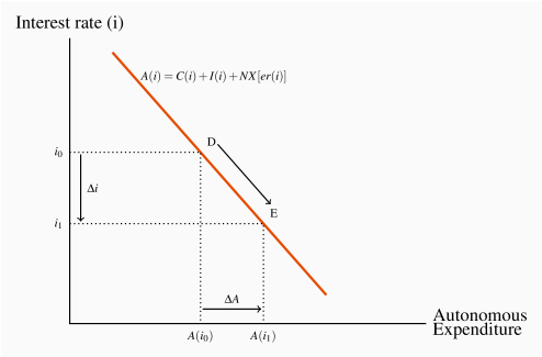
Figure 9.5 summarizes the relationship between interest rates and expenditures, assuming all things other than interest rates and exchange rates are constant. The downward sloping line A(i) illustrates the inverse relationship between the consumption, investment, and net export components of autonomous expenditure and the interest rate. Starting with interest rate i₀, the level expenditure related to interest rates is A(i₀), given by point D on the expenditure function. A fall in interest rates from i₀ to i₁ increases expenditure to A(i₁), moving along the expenditure function to point E. Lower interest rates increase consumption and investment expenditure directly through wealth and cost and availability of finance effects. Lower interest rates also increase net exports through the effects of lower interest rates on the foreign exchange rate. A rise in interest rates would have the opposite effect.

The changes in interest rates and exchange rates are the key linkages between the monetary and financial sector and aggregate demand.