We can now summarize and illustrate the relationships that transmit changes in money, financial markets, and interest rates to aggregate demand, output, and employment. There are four linkages in the transmission mechanism:
- With prices constant, changes in money supply change interest rates.
- Changes in interest rates change consumption expenditure through the wealth effect and the cost and availability of credit.
- Changes in interest rates also cause changes in planned investment expenditure through the cost and availability of credit to finance the purchase of capital equipment and to carry inventories.
- Changes in interest rates also cause changes in exchange rates, which change the price competitiveness and profitability of trade goods and services.
Working through these linkages, the effects of changes in money and interest rates on aggregate expenditure, aggregate demand and equilibrium real GDP is illustrated as follows:
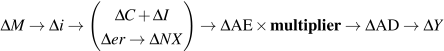
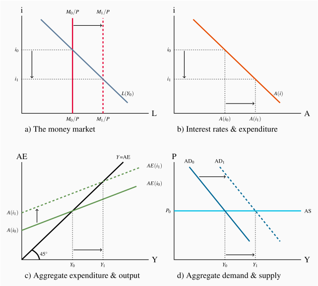
Figure 9.6 shows the transmission mechanism using four interrelated diagrams: a) the money market, b) interest rates and planned expenditure, c) aggregate expenditure and equilibrium output, and d) aggregate demand and supply, output, and prices. We continue to assume a constant price level, as the diagrams show. Changes in the money and financial sector affect aggregate demand and output, to add another dimension to our understanding of the sources of AD and fluctuations in AD.
To see the linkages in the transmission mechanism start in Panel a) with an equilibrium interest rate i0 determined by the initial money supply M0/P and demand for money L(Y0). This interest rate i0 induces autonomous expenditure A(i0) in Panel b). That autonomous expenditure is the vertical intercept A(i0) of the aggregate expenditure function  in Panel c), and through the multiplier the equilibrium GDP, Y0. In Panel d) the corresponding aggregate demand curve
  crosses the horizontal AS curve at the equilibrium real GDP Y0.
An increase in the money supply in Panel a) lowers equilibrium i to i1. This causes an increase in autonomous expenditure to A(i1) in Panel b) and an upward shift in the AE function on Panel c). Increased autonomous expenditure and the multiplier increase equilibrium real GDP and shift the AD curve to the right by the increase in A times the multiplier. The new equilibrium is Y1 at the price level P0.
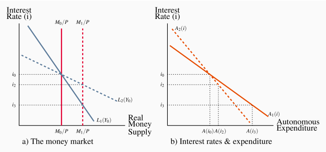
There are several key aspects to these linkages between money, interest rates, and expenditure. The effect of changes in the money supply on interest rates in the money market depends on the slope of the demand curve for real money balances. A steep curve would show that portfolio managers do not react strongly to changes in market interest rates. It would take relatively large changes in rates to get them to change their money balances. Alternatively, if their decisions were very sensitive to the interest rates, the L function would be quite flat. The difference is important to the volatility of financial markets and interest rates, which in turn affect the volatility of expenditure.
Panel a) in Figure 9.7 shows the effects of an increase in money supply under different money demand conditions.
The sensitivity of expenditure to interest rates and financial conditions is a second important aspect of the transmission mechanism. If the interest rate/expenditure function in Panel b) is steep, changes in interest rates will have only small effects on expenditure, aggregate demand, and output. A flatter expenditure function has the opposite implication.
Business cycles, output gaps, and policy issues
The effect of money and financial markets on expenditure, output, and employment raises two issues for macroeconomic policy. First, fluctuations in money supply and financial conditions are an important source of business cycle fluctuations in output and employment. These effects are particularly strong and important when the small changes in money supply have big impacts on interest rates and expenditure. A steep L(i) function and a flat expenditure/interest rate function would create these conditions. Stabilization policy would then need to control and stabilize the money supply, a policy approach advocated by monetarists, who see money supply disturbances as the major source of business cycles. If you can fix money supply at M0 in Figure 9.6, and the demand for money L(Y,i) and the interest rate/expenditure function are stable, you remove monetary disturbances as a source of business cycles.
This Monetarist approach to money and the financial sector concentrates on the "automatic" stabilization effects of money supply control. With the money supply fixed, any tendency for the economy to experience a recessionary or inflationary gap changes the demand for money, and interest rates change in an offsetting direction. A fall in real output that creates a recessionary gap reduces the demand for money L(Y,i) and, with a fixed money supply, interest rates fall to induce additional expenditure. An inflationary gap would produce an automatic rise in interest rates. The monetary sector automatically resists fluctuations in expenditure and output.
The second policy issue is the alternative to this approach. Discretionary monetary policy would attempt to manage money supply or interest rates or financial conditions more broadly. The objective would be to counter persistent autonomous expenditure and financial disturbances that create output gaps. The intent is to manage aggregate demand in an active way. In other words, if business cycles were caused by shifts and fluctuations in the interest rate/expenditure function in Panel b) of Figure 9.6, monetary policy would react by changing interest rates and money supply and move the economy along the new expenditure function to stabilize autonomous expenditure and aggregate demand. Keynesian and New-Keynesian economists advocate this active approach to policy in the money and financial sector, based on a different and broader view of the sources of business cycles in the economy.
Recent experience extends beyond these two policy concerns. A collapse in the financial sector on the supply side was a major cause of the recession of 2009. Banks and other financial institutions suffered losses on mortgages and other assets followed as energy and commodity prices dropped and expectations of business profits followed. Uncertainty on the part of many lenders about the quality of assets and the risks of lending reduced the availability of credit. Uncertainty on the part of households and businesses reduced their confidence in financial institutions. Although central banks worked to keep interest rates low and bank reserves strong, shifts in the availability of credit and the willingness to borrow shifted the A(i) curve in Figure 9.6 sharply to the left, expenditure fell, and AD shifted left, opening a strong recessionary gap that has been persistent in many industrial countries.
This recent experience has led to serious debates about the role and effectiveness of monetary policy and the objectives of fiscal policy. These are issues we examine in more detail in the chapters that follow.
Next
This chapter makes the link between money, interest rates, aggregate demand, and output in the model of the economy. It also shows that monetary policy, working through the monetary transmission mechanism, provides a second policy channel, in addition to fiscal policy, which government might use to stabilize business cycle fluctuations. Chapter 10 studies in detail the monetary policy operations of central banks, including the Bank of Canada.
Example Box 9.1 Bond prices and interest rates
Consider the price of the 4.25 percent bond with a maturity date of June 1, 2018. Let's assume that the 3 year market rate of interest on the date you buy the bond, say June 1, 2015 is 4.25 percent. The price of the bond is the present value of the future payments: $4.25 on June 1, 2016, $4.25 on June 1, 2017, and $104.25 on June 1, 2018. Payments to be received two years in the future are discounted twice, and three years in the future three times, to give:
A bond bought for $100 and held to maturity would yield 4.25 percent, the current market rate of interest assumed in this example. The bond is trading at par because the market price equals the face value.
As an alternative assume that the 3 year market rate of interest on June 1, 2015 is 1.75 percent. The price of the bond is then the present value of the future payments: $4.25 on June 1, 2016, $4.25 on June 1, 2017, and $104.25 on June 1, 2018. Payments to be received two years in the future are discounted twice, and three years in the future three times, to give:
The price of this 4.25 percent bond on June 1, 2018 would be $107.26 per $100 of face value. The assumption that the market rate of interest is 1.75 percent, which is clearly lower than the 4.25 percent coupon on the bond, means the bond trades at a premium. The premium price means that buying the bond and holding it to its maturity date will give an annualized return of 1.75 percent on your money. That is the then current assumed 3 year rate.
Taking account of the changes in bond prices as market interest rates change, the yield on the bond—the present value of its coupon payment plus the capital loss as its price falls to par at maturity—gives a rate of return equal to the market interest rate of 1.75 percent.
Application Box 9.1 A basic guide to financial assets
Three broad classes of financial assets are bought and sold in financial markets. These are bills, bonds, and equities.
Bills are short-term financial assets that make no interest payment to the holder but do make specified cash payment on their maturity date. They trade at a discount. A government treasury bill or T-Bill is an example. Every second week the government sells T-Bills that promise to pay the buyer $100 for each $100 of face value on the date that is about three months in the future. The interest earned is the difference between the price paid and the face amount received at the maturity date.
Bonds are longer-term financial assets that pay a fixed money income payment each year and repay their face value on a fixed maturity date. Bonds are marketable, and trade on the bond market between their issue dates and maturity dates at prices determined by supply and demand. As with T-Bills, the return to the holder of a bond depends on the price paid for the bond. In this case, the calculation is more complex however, because it involves a fixed annual money payment and a fixed value at maturity.
Equities are shares in the ownership of the business. They give the holder the right to a share in the profits of the business, either in the form of dividend payments or in terms of the increase in the size of the business if profits are used for business expansion. The shares or stocks in publicly traded businesses can be bought and sold on stock markets like the Toronto Stock Exchange. The financial pages of major newspapers give you daily reports on stocks prices and stock markets. Shareholders' returns from their stock holdings depend on the combination of dividend income they receive and the changes in the market price of the shares they hold. Equity prices are the expected value of the future profits of business. Because expectations of future business performance are volatile, equity prices are volatile and therefore risky. Equities do however offer the prospect of higher long-term returns.
Application Box 9.2 Nominal and real interest rates
Both nominal and real interest rates play important roles in the economy. The nominal (or money) interest rate is the annual percentage of the principal of a loan that the borrower pays to the lender. It is determined by supply and demand conditions in money markets. The real interest rate is the nominal interest rate adjusted for annual changes in the price level (real interest rate = nominal interest rate minus the inflation rate). When the inflation rate is zero, nominal and real interest rates are equal.
Nominal interest rates and financial asset prices are linked. The present value calculation of asset prices uses the nominal rate for discounting. Nominal interest rates and asset prices vary inversely.
Nominal interest rates also affect nominal cash flows of both households and businesses. A rise in nominal rates on lines of credit or mortgages increases the current cash cost of that borrowing. A fall in nominal rates on lines of credit or mortgages releases current cash commitments.
Real interest rates determine the real cost of borrowing and the real return to lending.
A family borrows $200,000 for one year at a nominal interest rate of 5 percent to buy a house. At the end of the year they would owe the lender $200,000 plus $10,000  interest. Their nominal interest cost is $10,000. If the price level has been constant over the year, their nominal interest cost and their real interest cost are equal at 5 percent.
Suppose however that the all prices are rising by 3 percent a year. The house bought today for $200,000 will sell for $206,000 one year from now. Borrowing at 5 percent to buy the house cost $10,000 but the rise in the price of the house by $6,000 offsets part of that cost. The real interest cost is  . The real interest rate is 2 percent based on the nominal interest rate of 5 percent minus the change in the price level of 3 percent.
With inflation rates greater than zero, lenders' real interest earnings are less than nominal interest earnings. In the preceding example, the mortgage lender's real return was just 2 percent  because the $210,000 received at the end of the year had its purchasing power reduced to approximately $204,000 by the 3 percent rise in the price level.
Nominal and real interest rates affect expenditure decisions by their effects on asset prices, cash flows, and the real costs and returns involved in borrowing and lending.