Growth in potential GDP measures the increase in the size of the economy, but it does not tell us what is happening to per capita GDP and standards of living. To discover the sources of growth in per capita GDP and improvements in standards of living, we need to study the production function in more detail. Then we can use growth accounting to uncover the sources of past growth in per capita GDP.
Factor contributions and scale economies
The increase in total output when an additional unit of a factor (labour or capital) is used in the production process, and other inputs are held constant, is the marginal product of that added factor. The production functions widely used in economics have diminishing marginal productivity. As more and more workers are employed using a fixed number of machines, each additional worker adds less and less to total output. The marginal product of labour, the change in total output as a result of using one more worker ( ), falls. Furthermore, because each additional input of labour adds less to total output than the unit before it, output per worker, Y/N, also falls.
Marginal product: the change in total output caused by a change of one unit in the input of that factor to production.
It is often assumed that production involves constant returns to scale. Instead of increasing just one input to production, suppose all inputs are increased together, in the same proportions. Labour and capital inputs might both be doubled, for example. Then, if output increases in exactly the same proportions as inputs have increased, there are constant returns to scale.
The production functions used in growth accounting have these properties. Consider the following example. Holding technology constant at A=1 to simplify matters, we can write:
 |
(13.4) |
using the weights we have used in growth accounting to measure the contributions of labour and capital to output, based on their shares in national income, as the exponents on labour and capital inputs. Table 13.4 gives numerical examples of the way this production function works.
The first row of the table shows that a labour input of 50 units combined with a capital input of 20 units gives output:

The next three rows illustrate the underlying diminishing returns and constant returns to scale in this production process. An increase of either labour input of 10 percent or capital input of 10 percent with the other input constant increases output, but by less than 10 percent in each case. Because output grows by less than the growth of the input in each case, output per worker or per unit of capital falls.
However, when only one input grows, output per unit of the factor held constant rises. In the second row of the table, capital input is constant when labour input grows. More labour inputs increase total output and output per unit of capital. Similarly, in the third row an increase in capital input increases labour productivity.
The fourth row of the table shows constant returns to scale. When labour and capital inputs both increase by the same proportion, output also increases by that proportion – 10 percent in this example. As a result, output per worker and output per unit of capital are constant. In terms of economic growth, equal growth rates of labour input and capital stock make total GDP grow at that same rate, but leave per capita GDP unchanged.
Constant returns to scale: equal percentage increases in inputs of labour and capital increase output by the same percentage.
To see the sources of growth in per capita GDP, we can manipulate the production function and apply growth accounting. To get per capita GDP, simply divide both sides of the production function in Equation 13.4 by N to give output per worker as follows:
 |
(13.4) |
Output per worker  , the number of workers employed.
To make the notation a bit neater, we can use lower case letters to indicate output per worker (y=Y/N) and capital per worker (k=K/N). This gives:
 |
(13.5) |
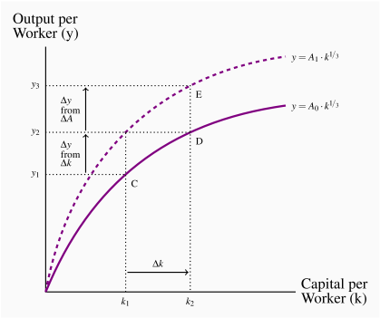
Figure 13.3 illustrates this production function in a diagram. The ratio of capital stock to labour, k, is measured on the horizontal axis. Output per worker, y, is measured on the vertical axis. Two per-worker production functions are used to distinguish between the effects of increases in capital stock and the effects of improvements in technology.
The declining slopes of both production functions illustrate the diminishing returns that lead to the smaller and smaller changes in output per worker as the capital/labour ratio increases. For example, starting at point C, an increase in the ratio of capital to labour moves the economy along the production function to point D. Output per worker increases at a decreasing rate. This shows that increased capital to labour ratios can increase output per worker until diminishing returns set in and limit sustained increases in output per worker. Sustained growth in per capita real GDP, in this basic model of growth, depends on improvements in technology to overcome the diminishing returns to increases in the capital to labour ratio.
Sustained growth in per capita real GDP: improvements in technology overcome the diminishing returns to increases in the capital to labour ratio.
An improvement in technology that increases productivity (A2>A1) shifts the production function up. At capital to labour ratio k2, for example, the increased productivity moves the economy from D to E as output per worker rises from y2 to y3. This shows that growth in per capita output, moving from y1 to y3, points C to E in Figure 13.3, is a result of both the growth in the capital to labour ratio and improvements in productivity.
Once again, growth accounting allows us to sort out the effects of these two factors on growth in output per worker and per capita GDP. Table 13.5 uses Canadian experience from 1990 to 2013 as an example.
Table 13.5 Sources of growth in per-worker GDP in Canada, 1990–2013
| |
Real |
Employ |
Capital |
Real |
Capital |
Growth |
Growth |
Contribution |
Solow |
| |
GDP |
N |
Stock K |
GDP |
per |
in Y/N |
in K/N |
from  |
Residual |
| |
Y |
(M) |
($B) |
per |
worker |
% |
% |
% |
% |
| |
($B) |
|
|
worker |
K/N |
|
|
|
|
| |
|
|
|
Y/N=y |
($K) |
|
|
|
|
| |
|
|
|
($K) |
|
|
|
|
|
| |
(1) |
(2) |
(3) |
(4) |
(5) |
(6) |
(7) |
(8)=(7)/3 |
(9)=(6)–(8) |
| 1990 |
993 |
13.1 |
1,427 |
75.98 |
109.18 |
– |
– |
– |
– |
| 1995 |
1,082 |
13.3 |
1,491 |
81.54 |
112.36 |
7.3 |
2.9 |
1.0 |
6.4 |
| 2000 |
1,328 |
14.8 |
1,603 |
89.97 |
108.60 |
10.3 |
–3.3 |
–1.1 |
11.5 |
| 2005 |
1,502 |
16.2 |
1,739 |
92.83 |
107.48 |
3.2 |
–1.0 |
–0.3 |
3.5 |
| 2013 |
1,698 |
17.7 |
2,094 |
95.99 |
118.37 |
3.4 |
10.1 |
3.4 |
0.0 |
Source: Statistics Canada, CANSIM Tables: 380-0106, 282-0087 and 031-0002 and author's calculations.
The first three columns of the table give data on real GDP, employment, and real capital stock for selected years over the 1990 to 2013 period. Columns (4) and (5) use these data to calculate the output per worker and capital per worker that we see in our per-worker production function. The growth in output per worker and the growth in capital per worker are reported in columns (6) and (7) as the percentage changes over three five-year periods and a final eight year period to use the latest data available.
Growth accounting divides the sources of growth in output per worker between increases in capital per worker and increases in productivity based on improvements in technology. From the production function, we know that an increase in the capital/labour ratio increases output per worker by a factor of 1/3. Column (8) in the table reports this weighted contribution of the increase in capital per worker to the increase we see in output per worker. Subtracting these contributions from the increases in output per worker gives the Solow residual, column (9), which again is a measure of the effect of improvements in technology on output per worker.
The 1990 to 2013 period is of interest because the Canadian experience provides different examples of growth in GDP per worker. In the first five years, 1990 to 1995, there was very little growth in employment but some growth in capital stock. As a result, the capital to labour ratio, k, increased by 2.9 percent and accounted for 1.0 percentage points, or 13 percent of the 7.3 percent growth in real GDP per worker. Improved technology as measured by the Solow residual contributed the other 6.4 percentage points.
By contrast, employment and capital stock both grew strongly from 1995 to 2000, but employment growth (11.2 percent) exceeded capital stock growth (7.6 percent). As a result, the growth in the capital to labour ratio was negative, at  percent. Nevertheless, output per worker grew more in the second period, up 10.3 percent. Productivity gains from improved technology, again measured by the Solow residual, were the major source of strong growth in GDP per worker.
The decline in the capital to labour ratio in the 1995 to 2000 period appears to have reduced the growth in output per worker in the 2000 to 2005 period. Even though capital stock increased by about 8 percent and employment grew by 9.5 percent, output per worker increased by only 3.2 percent over the period. The Solow residual in column (9) shows a very small contribution to growth in output per worker from improved technology.
In the final period, 2005–2013 the calculated Solow residual is zero. A strong increase in capital stock and the capital labour ratio explains all the observed growth in output per worker.
Thinking of these experiences in terms of the production functions in Figure 13.3 illustrates the differences between sub-periods. From 1990 to 1995, the economy moved to the right along the production function as k grew by 2.9 per cent, for example, from C to D in the diagram. This provided a 1.0 percent increase in y, as from y1 to y2. Improved technology shifted the production function up to further increase output per worker from y2 to y3 at point E in the diagram. In the next period, 1995 to 2000, the movement along the production function was in the opposite direction, to the left from E, as k declined. However, a very strong effect from improved technology as measured by the Solow residual of 11.5 percent shifted the production function upward (not shown in the diagram) and sustained the growth in output per worker at 10.3 percent.
These examples and the discussion of the sources of growth emphasize two key aspects of the growth process. One aspect is the growth in the stock of capital, which comes from the flow of savings and investment in the economy. The other is changing technical knowledge and technology of production. These are the keys to sustained growth in total output and standards of living, but their sources are more obscure than the sources of growth in capital stock. Indeed, pessimism about the fate of society was based on both the inadequacy of investment and stagnant technology.