Learn how to apply the supply and demand model to actual events
Define and calculate the neoclassical measure of social welfare
Investigate situations in which markets fail to produce desirable results
The Neoclassical Circular Flow Model
Because neoclassical economists are primarily interested in understanding and defending market capitalist systems, they require a basic model that describes how the various parts of such economies are linked together. The neoclassical circular flow model achieves this goal. To understand this model, it is first necessary to define more carefully what we mean by a market. People often use the term to refer to a physical location where buying and selling occurs. For example, people will speak of “going to the market.” Our definition of a market is much broader. It does refer to a coming together of buyers and sellers of a common good, service, or asset, but the buyers and sellers need not meet face to face. What is important is that they interact in some way through purchases and sales of a common item of exchange. For example, buyers and sellers may be spread out across the globe, interacting by computer only. Despite the distance between them, they participate in a market.
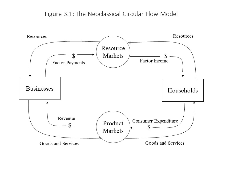
Given this definition of a market, we now turn to the neoclassical circular flow model represented in Figure 3.1.
As Figure 3.1 shows, the business sector and the household sector are linked together as a result of their interaction in two broad categories of markets. The first type of market is the resource market. Households own resources (or factors of production or inputs) that they sell to businesses. These resources include land, labor, and capital and so the major types of resource markets are the land, labor, and capital markets. The businesses use these resources to produce goods and services. In exchange for the resources, the businesses make factor payments to the households, which the households receive as factor income. For example, the payment for land generates rental income, the payment for labor generates wage income, and the payment for capital generates interest and profit income. The households use their factor income to purchase the goods and services that their resources produced in the second type of market referred to as the product market. The firms receive as revenue the consumer expenditure of the households.
Several important points need to be made about the circular flow model represented here. First, it should be noted that “real quantities” (i.e., resources and goods and services) flow in one direction in the diagram, and “nominal quantities” (i.e., dollar amounts) flow in the opposite direction.
Second, the model suggests that market economies are characterized by a strong element of social harmony. That is, buyers and sellers of resources and goods and services come together peacefully. Each gives up something he or she wants less than the thing obtained in exchange. Each market participant ends up better off at the end of each exchange than at the beginning. This world is the world of Adam Smith’s Invisible Hand in which self-interested individuals are guided as if by an invisible hand to promote the social interest. The process will continue indefinitely as long as buyers and sellers are allowed to interact freely in the marketplace.
Third, it is easy to be misled by the diagram into believing that market economies possess a rigid class structure. That is, one might interpret the model to mean that business owners confront members of households in the markets. In fact, the entire population is represented in the household sector. Remember, the household sector includes all resource owners, including the owners of land, labor, and capital. Even a person who owns no capital or land still owns his or her own labor, even if it is unskilled labor.
Who then, is included in the business sector? The answer is that any members of the household sector may decide to start up businesses. They simply enter the resource markets and purchase resources from other resource owners. They then establish businesses and sell the finished goods and services to other members of the household sector. Business owners sell goods and services, but they also purchase goods and services for their own consumption as members of the household sector. Similarly, they purchase resources as business owners, but they may even sell their resources in the resource markets as members of the household sector. If they use their own resources to establish their businesses, then they need not sell to themselves although they will expect to receive enough revenue to compensate themselves for the use of these self-owned resources. The important point here is that the owners of businesses need not be owners of capital or land who then purchase labor. They may just as easily be owners of labor who purchase capital and land. In other words, no resource owner has a privileged position within the economic system. As Paul Samuelson famously remarked, in a perfectly competitive market, it does not matter whether capital hires labor or labor hires capital.[1] Therefore, no class structure exists, and no class conflict is inherent in the model.
The Buyers’Side of the Market
Now that we have a detailed overview of the interconnections that exist within a market economy, we can begin to analyze the neoclassical theory of how markets function. The neoclassical theory of supply and demand has three parts: market demand, market supply, and marketequilibrium. Its purpose is to explain the two major outcomes of market competition: the price of the good, service or asset and the quantity exchanged of it. Before we combine the three parts of the model to show how they explain these two market outcomes, it will be helpful to provide a general overview of the method employed in the construction of the model. The method used is called methodological individualism. According to this approach, all social and economic outcomes are explained using individual actions. In terms of the supply and demand model, the starting point is individual buyers and individual sellers. Their actions are used to obtain the individual demands of the buyers and the individual supplies of the sellers. The individual demands are then aggregated (or summed up) to obtain market demand and the individual supplies are aggregated to obtain market supply. Finally, market demand and market supply are brought together to determine the market price and the market quantity exchanged. All these linkages are captured in Figure 3.2.
We will begin with the buyers’ side of the market first and discuss individual demand. The individual demand for a good is the amount of a good that a buyer is willing and able to buy at each price during a given period. It is important to note that both willingness and ability to pay are central to the definition of demand. If an individual lacks the dollars to back up his or her willingness to pay, then his or her preferences do not count in the marketplace. Furthermore, according to neoclassical economists, all consumers are subject to an economic law known as the law of demand. The law of demand states the following:
Other things equal, a reduction in price causes the quantity demanded of a good to rise, and a rise in price causes the quantity demanded of a good to fall.
In other words, price and quantity demanded are inversely related, ceteris paribus. This negative relationship can be represented symbolically as follows:[2]
We represent the individual demand for a good using an individual demand schedule and an individual demand curve, as shown in Figure 3.3.
The individual demand schedule shows clearly that the quantity demanded of apples (measured in pounds) per month rises as the price per pound of apples falls and vice versa. When the combinations of price and quantity demanded are plotted, we obtain a downward sloping individual demand curve. The downward slope implies that an inverse relationship exists between price and quantity demanded (i.e., that the law of demand holds).
At this stage, we have simply assumed that the law of demand holds, but it is important to understand why it is expected to hold. Neoclassical economists identify two reasons that we typically expect the individual demand curve to slope downwards:
As the price of apples declines, the consumer substitutes away from relatively higher priced goods, like bananas, and towards apples. This movement is known as the substitution effect. We might say that the consumer’s willingness to purchase apples has increased because it is relatively cheaper.
As the price of apples declines, the consumer feels that his or her purchasing power has increased and so he or she decides to purchase more of all goods, including apples. This movement is known as the income effect. We might say that the consumer’s ability to purchase apples has increased because his or her purchasing power has risen.
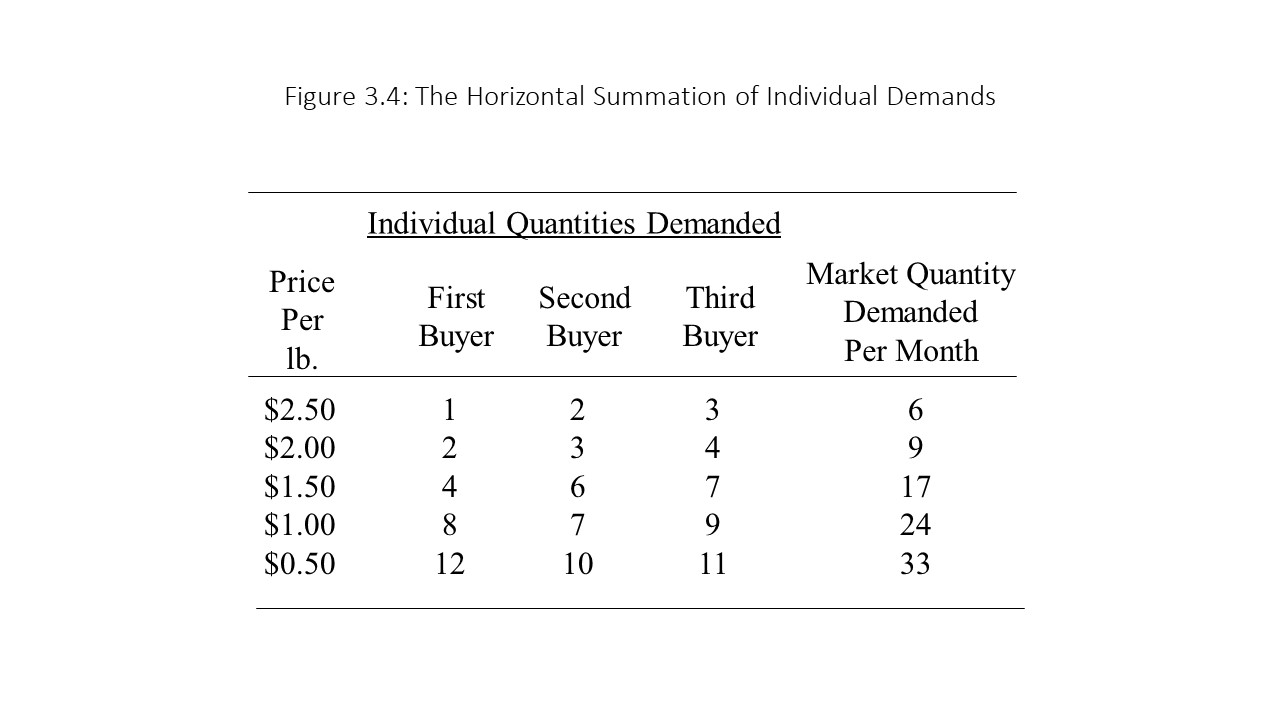
It is now possible to move from individual demand to market demand. Market demand refers to the quantity of a good that all buyers in a market are willing and able to purchase at each possible price during a given period. To obtain market demand, we must aggregate the individual demands of all individual buyers in the market. In terms of the individual demand schedules, we simply sum up the individual quantities demanded at each price to obtain the market quantity demanded at each price, as shown in Figure 3.4.
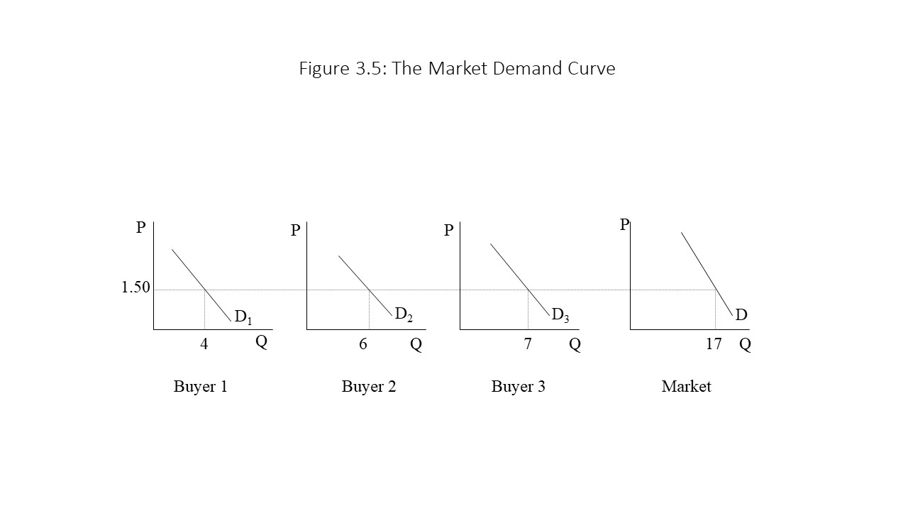
Graphically, this method of aggregation requires the summation of the horizontal distances from the vertical axis to the individual demand curve in each graph. For this reason, the method is referred to as horizontal summation. In Figure 3.5, this method is used to show the market quantity demanded at a price of $1.50. The other points on the market demand curve would be obtained in a similar fashion beginning with different prices.
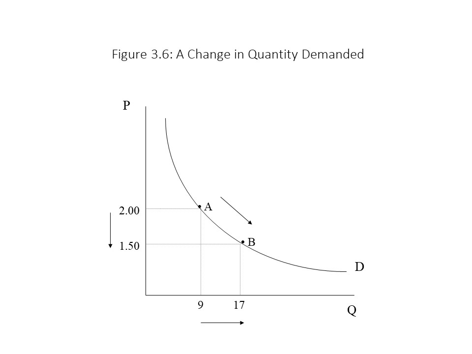
Now that we have obtained the market demand curve, it is time to introduce a key terminological distinction in the discussion of demand. Neoclassical economists distinguish between a change in quantity demanded and a change in demand. Figure 3.6 shows the downward sloping market demand curve for apples. As the price falls from $2.00 per lb. to $1.50 per lb., the quantity demanded of apples rises from 9 lbs. to 17 lbs. per month.
Such movements along the demand curve are referred to as changes in quantity demanded. In this case, the quantity demanded increases due to a price reduction. The quantity demanded also decreases when the price rises. It is important to note that the only factor that can cause a change in quantity demanded is a price change. In the case of the market demand curve, the price is the independent variable and the quantity demanded is the dependent variable. That is, the quantity demanded depends on the price. In mathematical terms, it is said that the quantity demanded is a function of the price of apples. That is:
Up until this point, we have acted as though the quantity demanded of a good depends only on the price charged for the good. Other factors are important to consumers as well, however, when they consider how much of a good to purchase. It is here that we begin to grasp the importance of the ceteris paribus assumption in the statement of the law of demand. The negative relationship between price and quantity demanded assumes that all other factors are held constant. If other factors change in addition to price, then this negative relationship may not hold. As a result, neoclassical economists assume that other factors are constant when tracing the demand curve. Nevertheless, neoclassical economists want to consider the possibility that other factors may change. These non-price determinants of demand include the following factors:
Consumer preferences or tastes
The number of buyers in the market
Consumers’ incomes
The prices of related goods
Consumer expectations about future prices
This list of factors implies that the quantity demanded of a product is a function of the good’s own price as well as all these other variables. That is:
The overbars indicate that these variables are held constant so that we can focus exclusively on the relationship between price and quantity demanded. When these variables change, however, the quantity demanded will be affected at every price. For example, Figure 3.7 shows what happens as Halloween approaches and the number of buyers in the market for apples increases.
The quantity demanded of apples at a price of $2/lb. rises from 9 lbs. per month to 26 lbs. per month. Similar increases in the quantity demanded occur at every possible price. As a result, the entire demand curve shifts to the right. Neoclassical economists refer to such a shift as an increase in demand (as opposed to an increase in quantity demanded). After Halloween, we might expect the quantity demanded of apples to fall at every price and the demand curve might shift to the left, back to its original position. Such a shift is referred to as a decrease in demand.
It is now possible to identify how changes in each of the non-price determinants of demand influence the demand curve. The case of a change in consumer preferences has already been discussed above in the context of a rise in the demand for apples:
Consumer preferences or tastes:
A strengthening of preference An increase in demand
A weakening of preference A decrease in demand
If more buyers enter a market, then the demand will also increase simply because it becomes necessary to aggregate a larger number of individual demands. If buyers exit the market, then fewer individual demands are aggregated and demand will decline.
The number of buyers in the market:
An increase in the number of buyers An increase in demand
A decrease in the number of buyers A decrease in demand
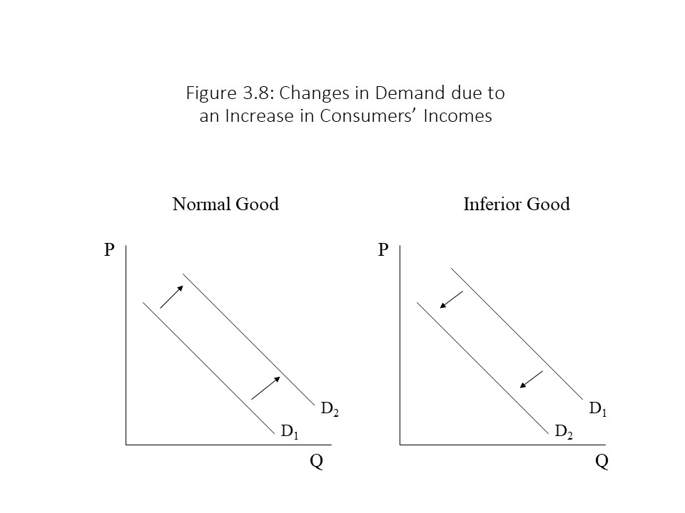
How changes in consumers’ incomes affect demand depends on how consumers perceive the good in question. The demands of many goods are positively related to income. If consumers experience a rise in their incomes, they demand more of the good. If consumers experience a reduction in their incomes, they demand less of the good. These goods are called normal goods. The demands of some goods, however, are negatively related to income. When consumers experience a rise in their incomes, they demand less of the good. When consumers experience a drop in their incomes, they demand more of the good. These goods are called inferior goods. The reader might wonder why a consumer would purchase more of a good as his or her income falls. Examples of inferior goods include used goods and generic goods. As consumers experience a fall in their incomes, they substitute away from new goods and brand name products and instead purchase used goods and generic products. Hence, we have the following results:
Consumers’ incomes:
An increase in the incomes of consumers of a normal good An increase in demand
A decrease in the incomes of consumers of a normal good A decrease in demand
An increase in the incomes of consumers of an inferior good A decrease in demand
A decrease in the incomes of consumers of an inferior good An increase in demand
Figure 3.8 shows how the market demand curves of normal and inferior goods are affected differently when incomes increase.
Changes in the prices of related goods may also cause changes in the demand for a good. If the price of a substitute for good A increases, for example, the demand for good A will rise, other things held constant. The reason is that consumers will substitute towards good A because it is now relatively cheaper. If the price of the substitute falls, then the demand for good A will fall as consumers substitute away from good A. For example, if the price of tea rises, we might expect the demand for coffee to rise as consumers switch from tea to coffee.
Alternatively, two goods may be complements in the sense that they are consumed together. If the price of a complement to good B increases, for example, then we would expect the demand for good B to fall, other things equal. If the price of a complement to good B falls, on the other hand, then we would expect the demand for good B to rise, other things equal. For example, if the price of peanut butter rises, then the demand for jelly will probably fall, other things equal. These results are summarized below:
Prices of related goods:
An increase in the price of a substitute An increase in demand
A decrease in the price of a substitute A decrease in demand
An increase in the price of a complement A decrease in demand
A decrease in the price of a complement An increase in demand
Finally, if consumers expect the price of a good to increase soon, then they frequently increase their demand for the good because they want to purchase the good before its price rises. For example, if consumers expect the price of gasoline to rise during Memorial Day weekend, they might demand more gasoline the weekend before that holiday to avoid paying the higher price. Alternatively, if the price is expected to fall in the future, then current demand will decline as consumers postpone their purchases in anticipation of a lower future price.[3]
Consumer expectations:
A rise in the expected price of gasoline An increase in demand
A fall in the expected price of gasoline A reduction in demand
The Sellers’ Side of the Market
We now turn to the sellers’ side of the market and discuss individual supply. (The reader will most likely notice a great many similarities between this discussion and the discussion of the buyers’ side of the market!) The individual supply of a good is the amount of a good that a seller is willing and able to sell at each price during a given period. According to neoclassical economists, all sellers are subject to an economic law known as the law of supply. In particular, the law of supply states the following:
Other things equal, an increase in price causes the quantity supplied of a good to rise, and a decrease in price causes the quantity supplied of a good to fall.
In other words, price and quantity supplied are positively related, ceteris paribus. This positive relationship can be represented symbolically as follows:
We represent the individual supply of a good using an individual supply schedule and an individual supply curve, as shown in Figure 3.9.
The individual supply schedule shows clearly that the quantity supplied of apples (measured in pounds) per month rises as the price per pound of apples rises and vice versa. When the combinations of price and quantity supplied are plotted, we obtain an upward sloping individual supply curve. The upward slope implies that a positive relationship exists between price and quantity supplied (i.e., that the law of supply holds).
At this stage, we have simply assumed that the law of supply holds, but it is important to understand why it is expected to hold. Neoclassical economists identify two reasons that we typically expect the individual supply curve to slope upwards:
As a firm increases production, the expansion puts upward pressure on per unit cost due to the scarcity of the firm’s resources. The firm requires a higher price to cover the higher unit cost of production.
As the price rises, the firm finds it profitable to produce additional units of the product. It eventually stops due to the rising unit costs mentioned above.
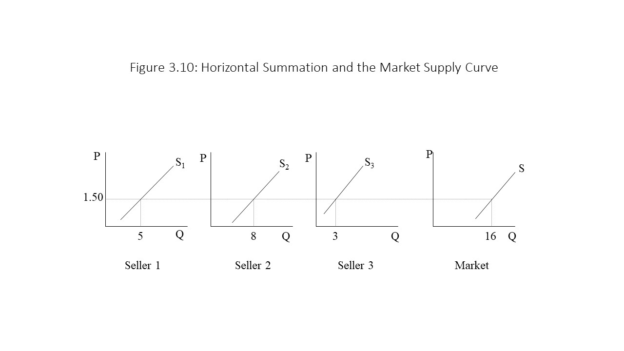
It is now possible to move from individual supply to market supply. Market supply refers to the quantity of a good that all sellers in a market are willing and able to sell at each possible price during a given period. To obtain market supply, we must aggregate the individual supplies of all individual sellers in the market. Just as in the case of demand, we use the method of horizontal summation. Graphically, this method of aggregation requires the summation of the horizontal distances from the vertical axis to the individual supply curve in each graph. In Figure 3.10, this method is used to show the market quantity supplied at a price of $1.50. The other points on the market supply curve would be obtained in a similar fashion beginning with different prices.
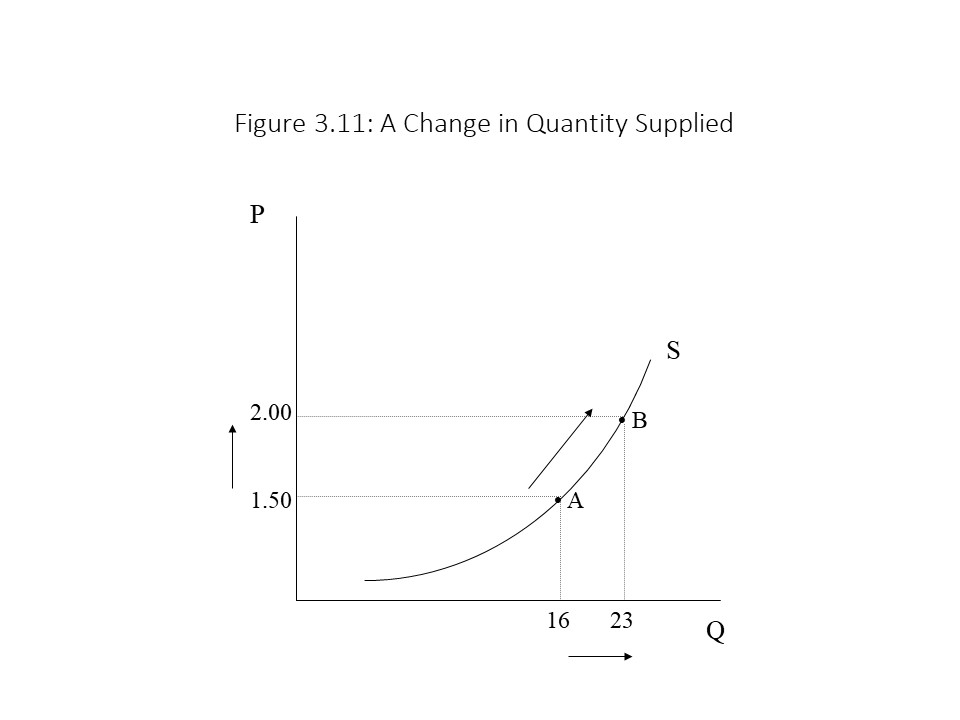
Now that we have obtained the market supply curve, it is time to reintroduce the key terminological distinction that arose in the discussion of demand. Neoclassical economists distinguish between a change in quantity supplied and a change in supply. Figure 3.11 shows the upward sloping market supply curve for apples. As the price rises from $1.50 per lb. to $2.00 per lb., the quantity supplied of apples rises from 16 lbs. to 23 lbs. per month.
Such movements along the supply curve are referred to as changes in quantity supplied. In this case, the quantity supplied increases due to a price increase. The quantity supplied also decreases when the price decreases. It is important to note that the only factor that can cause a change in quantity supplied is a price change. In the case of the market supply curve, the price is the independent variable and the quantity supplied is the dependent variable. That is, the quantity supplied depends on the price. In mathematical terms, it is said that the quantity supplied is a function of the price of apples. That is:
Up until this point, we have acted as though the quantity supplied of a good depends only on the price charged for the good. Other factors are important to sellers as well, however, when they consider how much of a good to sell. It is here that we should again recall the importance of the ceteris paribus assumption in the statement of the law of supply. The positive relationship between price and quantity supplied assumes that all other factors are held constant. If other factors change in addition to price, then this positive relationship may not hold. As a result, neoclassical economists assume that other factors are constant when tracing the supply curve. Nevertheless, neoclassical economists want to consider the possibility that other factors may change. These non-price determinants of supply include the following factors:
The number of sellers in the market
Factor prices
Production technology
Taxes and subsidies
The prices of related goods
The sellers’ expectations about future prices
This list of factors implies that the quantity supplied of a product is a function of the good’s own price as well as all these other variables. That is:
The overbars indicate that these variables are held constant so that we can focus exclusively on the relationship between price and quantity supplied. When these variables change, however, the quantity supplied will be affected at every price. For example, Figure 3.12 shows what happens in late summer and fall when apples are in season and thus the number of sellers in the market for apples increases.
The quantity supplied of apples at a price of $1.50/lb. rises from 16 lbs. per month to 22 lbs. per month. Similar increases in the quantity supplied occur at every possible price. As a result, the entire supply curve shifts to the right. Neoclassical economists refer to such a shift as an increase in supply (as opposed to an increase in quantity supplied). By late fall, we might expect the quantity supplied of apples to fall at every price and the supply curve might shift to the left, back to its original position. Such a shift is referred to as a decrease in supply.
It is now possible to identify how changes in each of the non-price determinants of supply influence the supply curve. The case of a change in the number of sellers has already been discussed above in the context of a rise in the supply of apples:
Number of sellers:
An increase in the number of sellers An increase in supply
A decrease in the number of sellers A decrease in supply
If factor prices change, then supply is affected. Factor prices (or resource prices or input prices) refer to the prices of land, labor, and capital. Specifically, if any of these factor prices rise causing rental payments, wage payments, or interest payments to rise, then firms will reduce their supply because their production costs have risen. Alternatively, if factor prices fall, then supply will rise because production costs are lower.
Factor prices:
An increase in factor prices A decrease in supply
A decrease in factor prices An increase in supply
Production technology is another important non-price determinant of supply. For example, when mass production methods were introduced in the automobile industry, production costs fell dramatically. Therefore, the supply of automobiles increased because firms could produce more at a given price. Although the implementation of an inferior technology is unlikely, it is theoretically possible and would lead to a reduction in supply as production costs rise.
Production technology:
A technological advance An increase in supply
The implementation of an inferior technology A decrease in supply
Changes in per unit taxes or subsidies on goods and services also influence product supply. For example, if the government increases the per unit tax on cigarettes, then production costs are higher and firms reduce the quantity supplied at every price. If the per unit tax on cigarettes falls, then firms increase their supply. Subsidies, on the other hand, have the opposite effect of taxes. Subsidies are cash payments that the government gives to sellers for each unit produced. If the government increases its subsidies for sellers, then production costs are effectively lower and product supply will rise. Alternatively, if the government cuts its subsidies to sellers, then product supply will fall.
Taxes and subsidies:
An increase in taxes A decrease in supply
A decrease in taxes An increase in supply
An increase in subsidies An increase in supply
A decrease in subsidies A decrease in supply
Prices of related goods sometimes also are important from the seller’s perspective. For example, if the same firms produce two different goods and each firm possesses a fixed amount of resources, then a change in the price of one good will affect the supply of the other good. For example, suppose that the same firms produce breath mints and chewing gum. If the price of breath mints increases, then it becomes relatively more profitable to produce breath mints, other factors held constant. Because firms possess fixed resources, they will reallocate resources towards breath mints and away from chewing gum. As a result, the supply of chewing gum decreases as shown in Figure 3.13.
Prices of related goods:
An increase in the price of another good the firm produces A decrease in supply
A decrease in the price of another good the firm produces An increase in supply
Finally, the expectations of producers about the future price may influence the supply of the product in a couple different ways.[4] For example, if the sellers expect the price to rise, then the sellers might expand supply now so that an increased quantity is present on the market when the price increase occurs. If they expect the price to fall, then supply might be reduced so that production is lower when the price decline occurs. On the other hand, a higher expected future price might lead sellers to store their current production and reduce supply. A lower expected future price might lead sellers to increase current supply so that they are able to sell before the price reduction.
Expectations about future prices:
A rise in the expected price An increase in supply (current expansion)
A fall in the expected price A reduction in supply (current contraction)
A rise in the expected price A decrease in supply (expansion of inventories)
A fall in the expected price An increase in supply (depletion of inventories)
Which outcome occurs depends on the circumstances related to the product. For example, durable goods can be stored for future sale whereas nondurable goods cannot be stored for long. Also, some price changes are expected soon whereas other price changes are expected in the distant future. The durability of the product and how soon the price change is expected are likely to interact to determine the impact on supply of an expected price change.
Equilibrium
We are almost to the point where we can combine the buyers’ side and the sellers’ side of the market to provide an explanation for the price and quantity exchanged of the product. Before we do so, we need to introduce a very important definition in neoclassical economics: equilibrium. The equilibrium concept is central to the theorizing of all neoclassical economists. Its definition is simple:
An equilibrium state refers to a state from which there is no inherenttendency to change.
To understand this definition, consider a non-economic example.[5] For example, imagine a bowl that has a marble resting on the edge. If the marble slips into the bowl, it will move down along the inside edge eventually reaching the bottom and then rising again along the opposite inside edge. From that point, it will slip back down again where it will reach the bottom and then rise again on the other side. This back and forth motion will continue until finally, the marble finds its position at the bottom of the bowl. Is this state an equilibrium state? Yes, it is. Notice that I can shake the bowl and cause the marble to move. Nevertheless, it is an equilibrium state because the marble has no inherent tendency to move from this point. In other words, the definition of equilibrium does not preclude the possibility that external shocks might cause a disruption.
Neoclassical economists argue that market prices and quantities exchanged reach equilibrium levels much like the marble in the example. How is such a thing possible? The answer becomes clear when we bring together market supply and market demand as shown in Figure 3.14.
To understand how the equilibrium price and quantity exchanged come about in this market, it is best to begin at a price that is not the equilibrium price. For example, suppose the price begins at $1.75 per unit. In that case, the quantity demanded is 0 units, but the quantity supplied is 18 units. Because sellers wish to sell 18 more units at this high price than buyers wish to buy, we say that an excess supply, or a surplus, of the good exists. Due to the surplus, sellers will feel pressure to cut price. Suppose that sellers cut the price to $1.50 per unit. As the price falls, the quantity demanded rises to 3 units due to the law of demand. Similarly, the quantity supplied falls to 15 units due to the law of supply. The result is a smaller surplus of 12 units (= 15 units – 3 units). The sellers will continue to feel pressure to cut price as long as a surplus exists. The reader should try to determine what the quantity demanded, the quantity supplied, and the surplus are at a price of $1.25 per unit.
Now consider what happens if the price begins at $0.25 per unit. In that case, the quantity supplied is 0 units, but the quantity demanded is 18 units. Because buyers wish to purchase 18 more units than are currently supplied, an excess demand, or a shortage, of the good exists. Due to the shortage, sellers will feel that they can increase the price. Suppose the sellers increase the price to $0.50 per unit. The quantity supplied will then rise to 3 units, according to the law of supply. Similarly, the quantity demanded will fall to 15 units due to the law of demand. The result is a smaller shortage equal to 12 units (= 15 units – 3 units). The sellers will continue to raise price if a shortage exists. The reader should try to determine the quantity demanded, the quantity supplied, and the amount of the shortage when the price rises to $0.75 per unit.
In the case of a shortage, the price will continue to rise until the price reaches $1.00 per unit. At this point, the quantity demanded is 9 units and the quantity supplied is 9 units. Therefore, neither a shortage nor a surplus exists in the market. As a result, sellers will not have an incentive to raise or lower the price. Every buyer who wishes to pay the current market price will be able to purchase the product, and every seller who wishes to sell at the current market price will be able to sell. All plans are consistent with one another. There is no inherent tendency for the price of $1.00 per unit or the quantity exchanged of 9 units to change. The outcome is, therefore, an equilibrium outcome. It is said that the market clears and so the equilibrium price and quantity are also referred to as the market-clearing price and quantity. These general results are summarized below:
It is very important to note that the equilibrium condition states that quantity supplied equals quantity demanded. It is false to express the equilibrium condition in terms of supply and demand being equal (S = D). If supply equals demand, then the supply and demand curves are identical. That is, supply and demand refer to the curves themselves, whereas quantity supplied and quantity demanded both refer to specific points on the curves.
One other point should be made about the forces at work that bring about the equilibrium outcome. In the case of the marble moving towards its equilibrium level at the bottom of the bowl, the force at work is gravity. What is the analogous force at work in the market? The answer is competition. When economists refer to market forces, they have in mind competition between buyers and sellers.
Comparative Statics Analysis
It was mentioned earlier that equilibrium states can be disrupted by external shocks. The external shocks that can disrupt the equilibrium market price and quantity are changes in the non-price determinants of demand and supply that were discussed previously. When such changes occur, the supply curve or the demand curve will shift, bringing about a new equilibrium outcome. The analysis that allows us to compare these static equilibrium states is known as comparative statics analysis.
Let us consider changes in the non-price determinants of demand. For example, in the years following the Second World War, Americans were eager to purchase automobiles and household appliances. They had been deprived of many material things due to the Great Depression of the 1930s and the wartime rationing. With the postwar economic boom, many Americans experienced rising incomes, and they were ready to spend. Because these goods were normal goods, the demand for these goods rose. Figure 3.15 (a) shows the effect of an increase in demand on the market price and quantity exchanged for a good.
To understand how the movement from one equilibrium point to another occurs, it is useful to break up the movement into three steps. The first step is to identify whether supply or demand shifts and in which direction. The second step is to explain whether a surplus or a shortage exists at the initial equilibrium price of P1. The third and final step is to explain the direction of the changes in price and quantity exchanged.
Figure 3.15 (b) shows what happens in the market for apples when the number of buyers decreases in late fall. The reduction in demand causes a surplus, which then causes the price and quantity exchanged to decline.
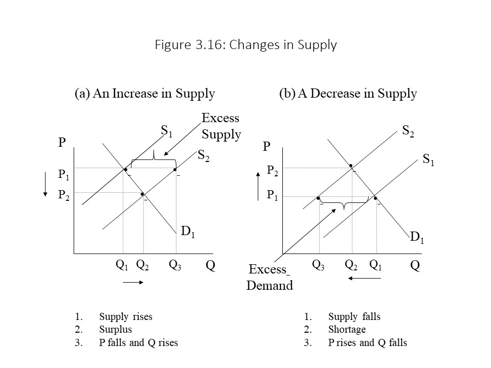
Similarly, Figure 3.16 (a) shows the effect of an increase in supply, which might occur due to a reduction in per unit taxes on cigarettes. Such a change creates a surplus and causes the price to fall and the quantity exchanged to rise. On the other hand, if a shortage of steelworkers causes wages to rise in the steel industry, then the rise in factor prices will lead to a reduction in the supply of steel as shown in Figure 3.16 (b).
Simultaneous Shifts in Supply and Demand
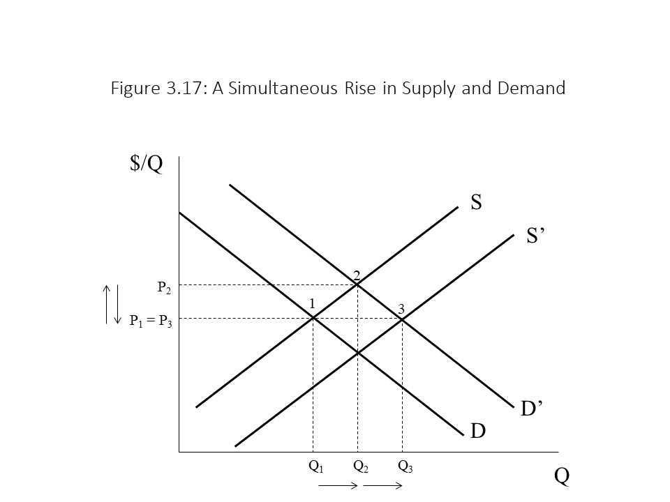
Each of the cases discussed in the previous section involves a shift in supply or demand only. It is possible, however, that both supply and demand might shift simultaneously. For example, the supply of oil might increase due to the development of new production technologies while the demand for oil increases as developing nations become more industrialized. This case is illustrated in Figure 3.17.
Based on the figure, it is clear that an increase in demand raises the equilibrium price and quantity exchanged. The equilibrium point moves from point 1 to point 2. The increase in supply, however, causes the equilibrium price to fall and the quantity exchanged to rise further. The final equilibrium point is at point 3. In this case, the reader can see that the quantity exchanged must rise because both factors contribute to a higher equilibrium quantity. On the other hand, the equilibrium price rises but then falls again. In this case, the price returns to its former level. One can easily imagine, however, a slightly larger increase in supply. Such a change would cause an overall reduction in price. Alternatively, a slightly smaller increase in supply would lead to an overall rise in price. The point is that unless we know the magnitudes of the shifts in supply and demand, we cannot determine whether price rises, falls, or stays the same overall. Our general conclusion, in this case, is that the quantity exchanged must rise, but the change in price is indeterminate (i.e., cannot be determined).
It turns out that in all four of the possible cases involving simultaneous shifts in supply and demand, the change in one of the variables (i.e., price or quantity) will be known for sure, and the change in the other variable will be indeterminate. The four possibilities are summarized below:
Supply and demand both rise: Q must rise but ∆P is indeterminate
Supply and demand both fall: Q must fall but ∆P is indeterminate
Supply rises and demand falls: P must fall but ∆Q is indeterminate
Supply falls and demand rises: P must rise but ∆Q is indeterminate
The reader should draw the graphs for cases 2-4, perhaps with the help of an instructor.
The Measurement of Social Welfare
We have been discussing the determination of the equilibrium price and quantity exchanged using supply and demand analysis. Neoclassical economists are also interested in measuring how well-off consumers and producers are when the market is in equilibrium. To measure the well-being of consumers and producers, neoclassical economists use the concepts of consumers’ surplus and producers’ surplus, respectively. We will consider each concept in turn.
Consumers’ surplus refers to the difference between the maximum amount that consumers are willing and able to pay for a good and the amount they do pay for it.
For example, if you go to the mall to purchase a shirt, you may be willing and able to pay as much as $30 for the shirt. Because the price on the tag (the market price) is only $20, however, you enjoy the $10 difference in the sense that you acquire the shirt, and you retain the additional $10 that you would have been willing and able to pay. This surplus that the consumer enjoys is a measure of how well-off he or she is.
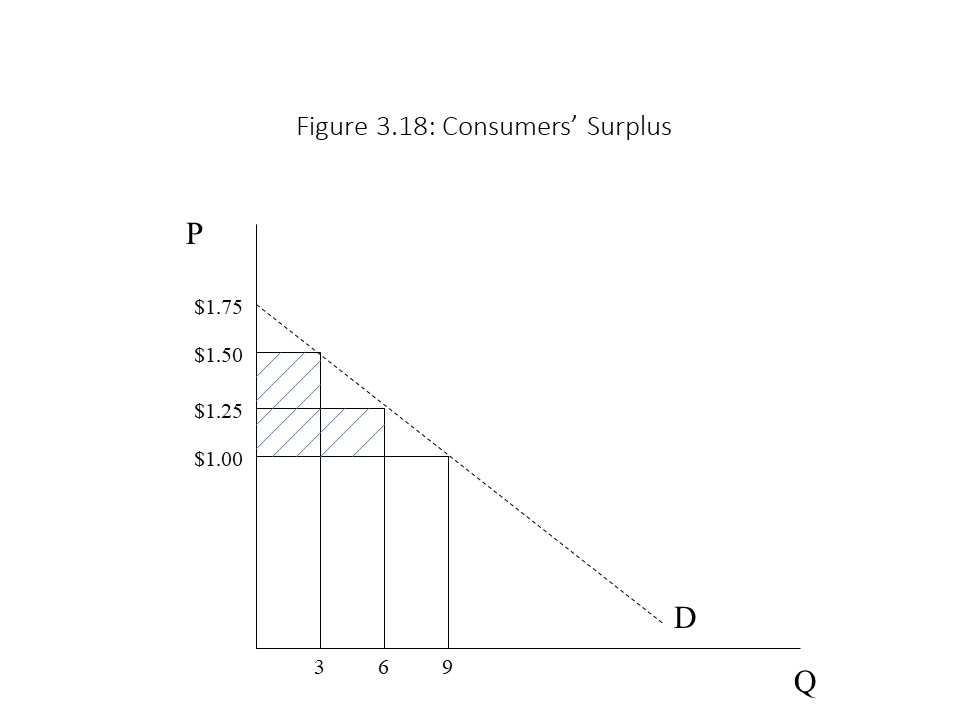
To calculate consumers’ surplus for the entire market, we only need to recall the fact that the market demand curve represents the maximum prices that consumers are willing and able to pay for a good. Furthermore, because consumers pay the market price for the good, the consumers’ surplus can always be represented as the area below the demand curve and above the current market price. Figure 3.18 shows how to approximate consumers’ surplus by treating the demand curve as if it possesses a staircase shape. The shaded area represents this approximation of the consumers’ surplus given the current market price of $1.00 per unit.
To calculate the consumers’ surplus using this approach, it is only necessary to add up the shaded areas. We add the surplus of $0.50 on each of the units from 0 to 3, the surplus of $0.25 on each of the units from 3 to 6, and the surplus of $0.00 on the units from 6 to 9.
To calculate the consumers’ surplus exactly, it would be necessary to include the entire area below the demand curve and above the price line. It should be clear that a larger area implies a greater welfare for consumers because the difference between the amount they are willing and able to pay and the amount they do pay is larger. The reader should also note that consumer expenditure is equal to $9.00 (= $1.00 per unit times 9 units).
We now turn to the related concept of producers’ surplus. It is defined as follows:
Producers’ surplus refers to the difference between the amount that producers receive for a good and the minimum amount producers are willing and able to accept.
To calculate producers’ surplus for the entire market, we only need to recall the fact that the market supply curve represents the minimum prices that producers are willing and able to accept for a good that they are selling. Furthermore, because producers receive the market price for the good, the producers’ surplus can always be represented as the area above the supply curve and below the current market price. Figure 3.19 shows how to approximate producers’ surplus by treating the supply curve as if it possesses a staircase shape. The shaded area represents this approximation of the producers’ surplus given the current market price of $1.00 per unit.
To calculate the producers’ surplus using this approach, it is only necessary to add up the shaded areas. We add the surplus of $0.50 on each of the units from 0 to 3, the surplus of $0.25 on each of the units from 3 to 6, and the surplus of $0.00 on the units from 6 to 9.
To calculate the producers’ surplus exactly, it would be necessary to include the entire area below the price line and above the supply curve. It should be clear that a larger area implies a greater welfare for producers because the difference between the amount they receive and the minimum amount they are willing and able to receive is larger. The reader should also note that the revenue that producers receive is equal to $9.00 (= $1.00 per unit times 9 units). It should also be noted that the revenue that producers receive is equal to the expenditure of consumers. This result is perfectly consistent with the neoclassical circular flow diagram represented in Figure 3.1.
Although the concepts of consumers’ surplus and producers’ surplus have been represented here as being entirely consistent with the neoclassical worldview, we will consider two very important criticisms of these concepts in chapter 6.
The Economic Efficiency of Competitive Markets
We now come to an important conclusion that neoclassical economists draw. According to neoclassical economists, competitive markets achieve economic efficiency, as defined in chapter 2. In chapter 2, it is explained that a society achieves economic efficiency when it achieves productive efficiency, allocative efficiency, and full employment. Another way of thinking about economic efficiency is in terms of the maximization of consumers’ surplus and producers’ surplus. The total surplus (TS) is simply the sum of consumers’ surplus and producers’ surplus. When it is maximized, economic efficiency is achieved. Neoclassical economists argue that total surplus is maximized when the market is in equilibrium.
To understand their reasoning, we must take a slight detour into the analysis of government intervention in the marketplace. Suppose, for example, that the government imposes a price ceiling in the market for gasoline. A price ceiling is a maximum legal price that may be charged for a good or service. If the equilibrium price in the market for gasoline is $3.75 per gallon and the price ceiling is set at $3.25 per gallon, then the situation in Figure 3.20 is the result.
Because the price is prevented from rising above $3.25 per gallon, a shortage equal to Q2 – Q1 is the result. Furthermore, the shortage will persist indefinitely unless something else changes. The efficiency implications of the price ceiling are of even greater interest. Because only Q1 units of output are supplied at the low price, the consumers’ surplus and producers’ surplus on units Q* – Q1 are simply lost. This loss of surplus is referred to as deadweight loss. Therefore, any price set below the equilibrium price will reduce the total surplus realized in the market.Figure 3.21 is the result.
Because the price is prevented from falling below $4.00 per gallon, an excess supply equal to Q2 – Q1 is the result. Furthermore, the excess supply will persist indefinitely unless something else changes. The efficiency implications of the price floor are of great interest just as in the case of the price ceiling. Because only Q1 units of output are demanded at the high price, the consumers’ surplus and producers’ surplus on units Q* – Q1 are simply lost. As in the case of the price ceiling, deadweight loss is the result. Therefore, any price set above the equilibrium price will reduce the total surplus realized in the market.
For price floors to be effective or binding, they must be placed above the equilibrium price. A price floor set below the equilibrium price would not have any effect on the marketplace because price has no tendency to fall that low. Price will simply move to its equilibrium level. Similarly, price ceilings must be placed below the equilibrium price if they are to be binding. A price ceiling set above the equilibrium price would have no effect on the market participants. The price would simply fall to its equilibrium level because a price ceiling does not prohibit downward movements in price.
Maximum efficiency is, therefore, equivalent to maximization of total surplus and is achieved when the market reaches equilibrium. Any price charged other than the equilibrium price leads to deadweight loss. At the societal level, it is possible to understand how market equilibrium leads to economic efficiency in a different way. Specifically, economic efficiency requires full employment of resources, productive efficiency, and allocative efficiency. If each resource market clears, then the entire quantity supplied of each resource will also be demanded. As a result, full employment will be achieved. In addition, if we interpret the supply curve as representing the marginal cost (MC) of production and the demand curve as representing the marginal benefit (MB) of a good, then the equilibrium outcome implies that MB = MC, which is the condition for allocative efficiency. Unfortunately, we must wait until chapter 8 for a demonstration that market equilibrium leads to productive efficiency (or least-cost production).
The Possibility of Market Failure
It has been shown that free and unfettered markets lead to economic efficiency or the maximization of consumers’ and producers’ surplus. We now ask whether exceptions to this general rule can be found. When competition in the marketplace fails to bring about economic efficiency, we call this situation market failure. Several types of market failure have been identified. In this section, we briefly explore two broad types of market failure.
The first kind of market failure occurs with the production of public goods. Public goods are goods that have two key characteristics: non-rivalry and non-excludability. A good is non-rival if one individual’s consumption of the good does not in any way reduce another individual’s consumption of the good. The classic example is a lighthouse. Once the lighthouse is constructed and operational, all boats entering a harbor enjoy the benefit of the light, and one boat’s consumption of the light does not diminish another boat’s consumption of the light. By contrast, a private good, like a sandwich, is a rival good because one individual’s consumption necessarily reduces another individual’s consumption.
A lighthouse also has the characteristic of non-excludability. That is, it is not possible to exclude any one boat from consuming the service that the lighthouse provides once it is operating. As a result, if the lighthouse owner wishes to charge a fee for the use of the lighthouse, it will not be possible to do so. That is, a boat can consume the service without paying.
This situation creates a free-rider effect in the sense that each boat has an incentive to free ride on the efforts of other boat owners to pay for the construction of the lighthouse. Because all boat owners face this same situation, no one is willing to pay for the construction of the lighthouse, and it is not built even though the benefit to the boat owners outweighs the cost of construction. Therefore, the market fails to deliver the efficient amount of the good, and so it is a case of market failure. The case is frequently made that the government can enhance efficiency in these situations by imposing a tax on the boat owners to force the collection of the fees that would be needed to build the lighthouse.
The other kind of market failure that we will consider is referred to as an externality. Externalities are external effects of a market transaction on third parties that are not directly involved in the transaction. Externalities may be positive or negative. For example, a negative externality may occur when a steel company dumps waste into a nearby river. The waste imposes a cost on those living down the river. The price of steel, however, will not reflect this cost because it is not part of the private cost of production for the steel company. Neither the buyers nor the sellers of steel will experience the negative effects of this added cost of production. This situation is depicted in Figure 3.22 where MPC represents marginal private cost, MSC represents the marginal social cost of production, and MPB represents the marginal private benefit. The MSC includes both the MPC and the external cost of pollution. For this reason, the MSC is higher than the MPC.
In Figure 3.22, the market clears at P* and Q*. The efficient outcome, however, occurs where MPB intersects MSC at P1 and Q1. Because the efficient outcome occurs at a higher price and a lower quantity, the implication is that the good is under-priced and over-produced in a competitive market. The case might be made that a unit tax imposed on producers can be used to reduce supply and bring it into line with MSC. Such a tax is known as a Pigouvian tax after the economist A.C. Pigou.[6]
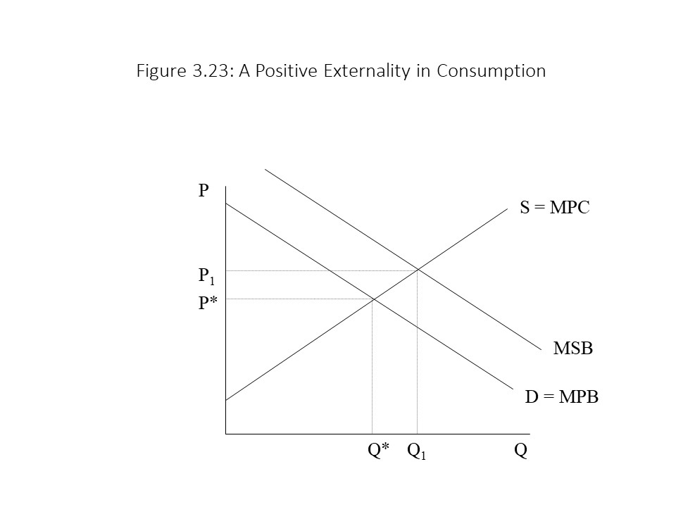
On the other hand, a positive externality may occur when consumption of a good leads to benefits for third parties that are not directly involved in the market transaction. For example, education is a good that is often argued to have positive spillover benefits in that other members of society benefit when people have more education rather than less. For example, a better educated population will have higher earning potential and so is less likely to resort to crime. Therefore, the marginal social benefit (MSB) exceeds the MPB in this case because the MSB includes the benefits that third parties receive in addition to the private benefits received by the direct consumers of education. This situation is depicted in Figure 3.23.
In Figure 3.23, the market clears at P* and Q*. The efficient outcome, however, occurs where MSB intersects MPC at P1 and Q1. Because the efficient outcome occurs at a higher price and a higher quantity, the implication is that the good is under-priced and under-produced in a competitive market. The case might be made that a subsidy per unit given to consumers can be used to increase demand and bring it into line with MSB. Of course, it is difficult to know just how much of a tax or subsidy to impose in these cases of market failure. An error might lead to an even greater inefficiency than the one resulting in the case of competitive equilibrium.
In July 2019, The Australian reported that the price of thermal coal fell significantly during the previous year. According to Nick Evans, Whitehaven Coal experienced a 25% reduction in the price of the coal it sells. Evans identifies a couple reasons for the significant reduction in coal prices. First, reductions in the demand for Australian coal exports hit Australian producers of coal hard. The lower foreign demand for Australian coal led to downward pressure on coal prices. A second factor that contributed to the lower coal prices is “tumbling gas prices.” Because gas is a substitute for coal, when gas prices fall, the demand for substitutes like coal falls. This factor has contributed to the lower demand for coal and to the lower coal prices. Despite the downward pressure on coal prices, Evans explains that coal prices are expected to moderate. The reason is that high-cost producers of coal will be driven out of business due to the low price of coal. Other high-cost producers, even if not forced to close, will cut production in response to the lower coal prices. As market supply contracts in the industry, upward pressure on the price occurs. If supply contracts sufficiently, then it may offset the reductions in demand and allow the market price of coal to stabilize. This case offers a good example of a complex case in which both supply and demand shift. The overall impact on the price in this case will be indeterminate. That is, the price may rise, fall, or remain the same overall, but the quantity exchanged in the market is sure to fall, as both the reduction in market demand and the reduction in market supply reduce the quantity exchanged in the market.
Summary of Key Points
The neoclassical circular flow model represents the linkages between the business sector and the household sector as harmonious and without class antagonisms.
The law of demand states, that other factors held constant, price and quantity demanded are inversely related.
A change in quantity demanded is due to changes in price only whereas a change in demand is due to changes in non-price determinants of demand.
The law of supply states, that other factors held constant, price and quantity supplied are positively related.
A change in quantity supplied is due to changes in price only whereas a change in supply is due to changes in non-price determinants of supply.
In market equilibrium, quantity supplied equals quantity demanded and neither a shortage nor a surplus exists.
Changes in the non-price determinants of demand and supply lead to changes in equilibrium prices and quantities exchanged.
Market equilibrium leads to the maximization of consumers’ surplus and producers’ surplus.
Binding price ceilings and binding price floors prevent the movement to equilibrium and reduce consumers’ surplus and producers’ surplus.
Market failures occur when markets fail to achieve economic efficiency.
List of Key Terms
Neoclassical circular flow model
Market
Resource market
Product market
Market demand
Market supply
Market equilibrium
Methodological individualism
Individual demands
Individual supplies
Law of demand
Substitution effect
Income effect
Horizontal summation
Change in quantity demanded
Change in demand
Normal goods
Inferior goods
Substitutes
Complements
Law of supply
Change in quantity supplied
Change in supply
Taxes
Subsidies
Equilibrium
Excess supply
Surplus
Excess demand
Shortage
Comparative statics analysis
Consumers’ surplus
Producers’ surplus
Total surplus
Price ceiling
Deadweight loss
Price floor
Effective or binding (price ceilings and price floors)
Market failure
Public goods
Free rider effect
Externalities
Marginal private cost (MPC)
Marginal social cost (MSC)
Marginal private benefit (MPB)
Pigouvian tax
Marginal social benefit (MSB)
Problems for Review
Suppose the price of peanut butter falls. If P1 and Q1 are the current equilibrium price and quantity of jelly, then how will the jelly market be affected by the drop in the price of peanut butter? Analyze this case in three steps.
Suppose the unit tax on gasoline is reduced. If P1 and Q1 are the current equilibrium price and quantity of gasoline, then how will the gasoline market be affected by the drop in the unit tax? Analyze this case in three steps.
Suppose consumers of an inferior good experience a rise in their incomes. If P1 and Q1 are the current equilibrium price and quantity of this good, then how will the market be affected by the rise in incomes? Analyze this case in three steps.
Suppose the demand rises for a good while the supply falls. Which conclusions can be drawn about the overall effect on equilibrium price and quantity exchanged? How would you draw the graph of this case?
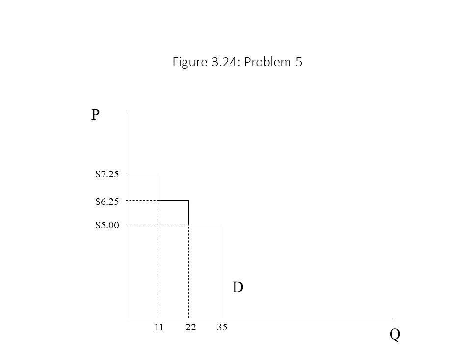
Suppose the price of the good in Figure 3.24 is $5 per unit. Calculate the consumers’ surplus using the information in the graph.
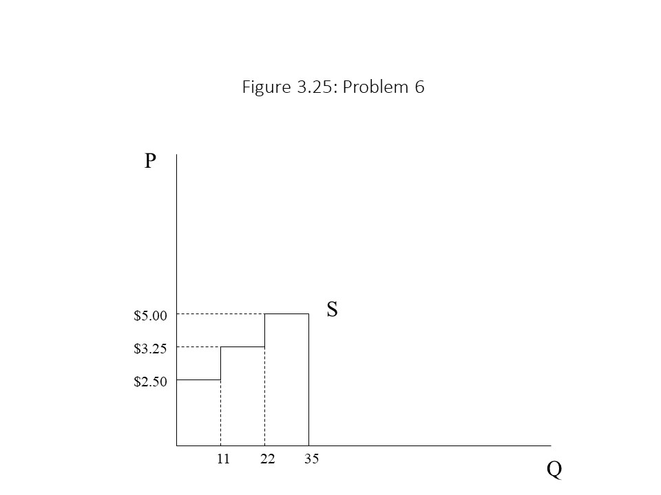
Suppose the price of the good in the graph below is $5 per unit. Calculate the producers’ surplus using the information in the graph.
Samuelson, Paul. 1957. “Wages and Interest: A Modern Dissection of Marxian Economic Models.” American Economic Review, 47: 884, 894. ↵
This notation follows notation that Prof. David Ruccio used in his undergraduate economics principles class at the University of Notre Dame during my years as his teaching assistant in the early 2000s. ↵
The reader should note that a movement along the demand curve does not occur in this case because the price of gasoline has not yet changed. It is only the expected future price of gasoline that has changed. ↵
McConnell and Brue (2008), p. 52, recognize both possible outcomes whereas many authors of neoclassical textbooks only emphasize the case of current storage. ↵
I believe that I first encountered this example in Prof. Kevin Quinn’s introductory economics class at BGSU. ↵
For a nice summary of how externalities violate the neoclassical efficiency theorem and different approaches to resolving them, see Rosser and Rosser (2004), p. 32-36. ↵
Evans, Nick. “Whitehaven tips steadier coal price as high-cost producers exit.” The Australian. Australian edition. 12 July 2019. ↵


 As Figure 3.1 shows, the business sector and the household sector are linked together as a result of their interaction in two broad categories of markets. The first type of market is the resource market. Households own resources (or factors of production or inputs) that they sell to businesses. These resources include land, labor, and capital and so the major types of resource markets are the land, labor, and capital markets. The businesses use these resources to produce goods and services. In exchange for the resources, the businesses make factor payments to the households, which the households receive as factor income. For example, the payment for land generates rental income, the payment for labor generates wage income, and the payment for capital generates interest and profit income. The households use their factor income to purchase the goods and services that their resources produced in the second type of market referred to as the product market. The firms receive as revenue the consumer expenditure of the households.
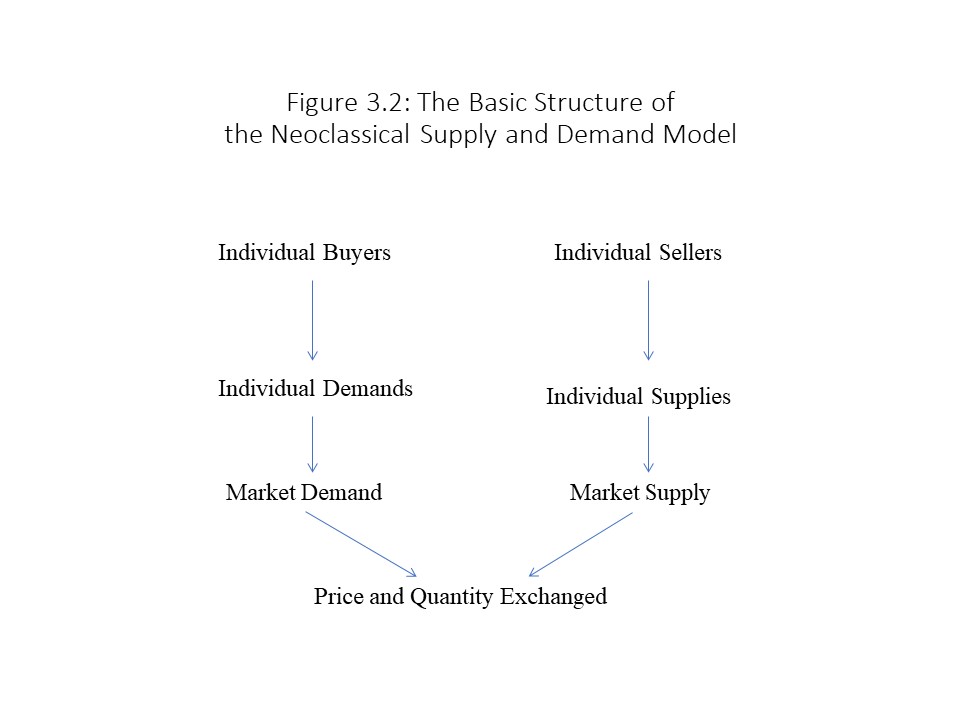 We will begin with the buyers’ side of the market first and discuss individual demand. The individual demand for a good is the amount of a good that a buyer is willing and able to buy at each price during a given period. It is important to note that both willingness and ability to pay are central to the definition of demand. If an individual lacks the dollars to back up his or her willingness to pay, then his or her preferences do not count in the marketplace. Furthermore, according to neoclassical economists, all consumers are subject to an economic law known as the law of demand. The law of demand states the following:
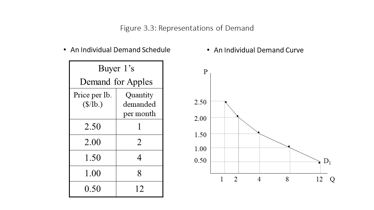
 Such movements along the demand curve are referred to as changes in quantity demanded. In this case, the quantity demanded increases due to a price reduction. The quantity demanded also decreases when the price rises. It is important to note that the only factor that can cause a change in quantity demanded is a price change. In the case of the market demand curve, the price is the independent variable and the quantity demanded is the dependent variable. That is, the quantity demanded depends on the price. In mathematical terms, it is said that the quantity demanded is a function of the price of apples. That is:
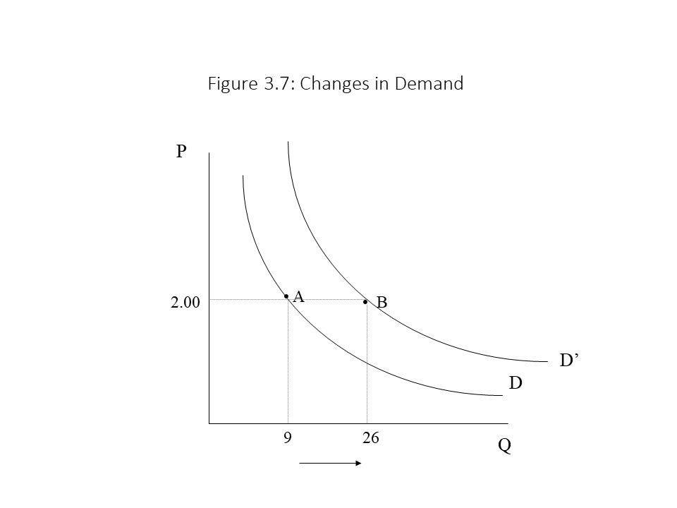 The quantity demanded of apples at a price of $2/lb. rises from 9 lbs. per month to 26 lbs. per month. Similar increases in the quantity demanded occur at every possible price. As a result, the entire demand curve shifts to the right. Neoclassical economists refer to such a shift as an increase in demand (as opposed to an increase in quantity demanded). After Halloween, we might expect the quantity demanded of apples to fall at every price and the demand curve might shift to the left, back to its original position. Such a shift is referred to as a decrease in demand.
An increase in demand
 Changes in the prices of related goods may also cause changes in the demand for a good. If the price of a substitute for good A increases, for example, the demand for good A will rise, other things held constant. The reason is that consumers will substitute towards good A because it is now relatively cheaper. If the price of the substitute falls, then the demand for good A will fall as consumers substitute away from good A. For example, if the price of tea rises, we might expect the demand for coffee to rise as consumers switch from tea to coffee.
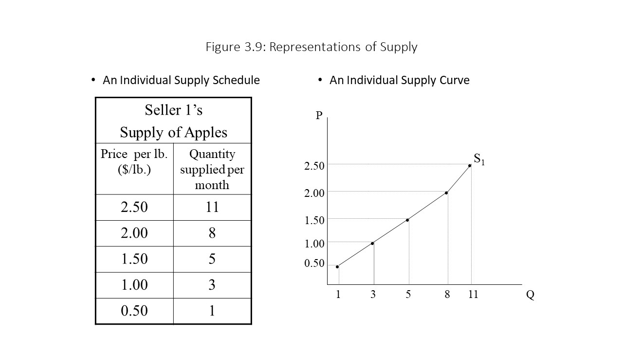
 Such movements along the supply curve are referred to as changes in quantity supplied. In this case, the quantity supplied increases due to a price increase. The quantity supplied also decreases when the price decreases. It is important to note that the only factor that can cause a change in quantity supplied is a price change. In the case of the market supply curve, the price is the independent variable and the quantity supplied is the dependent variable. That is, the quantity supplied depends on the price. In mathematical terms, it is said that the quantity supplied is a function of the price of apples. That is:
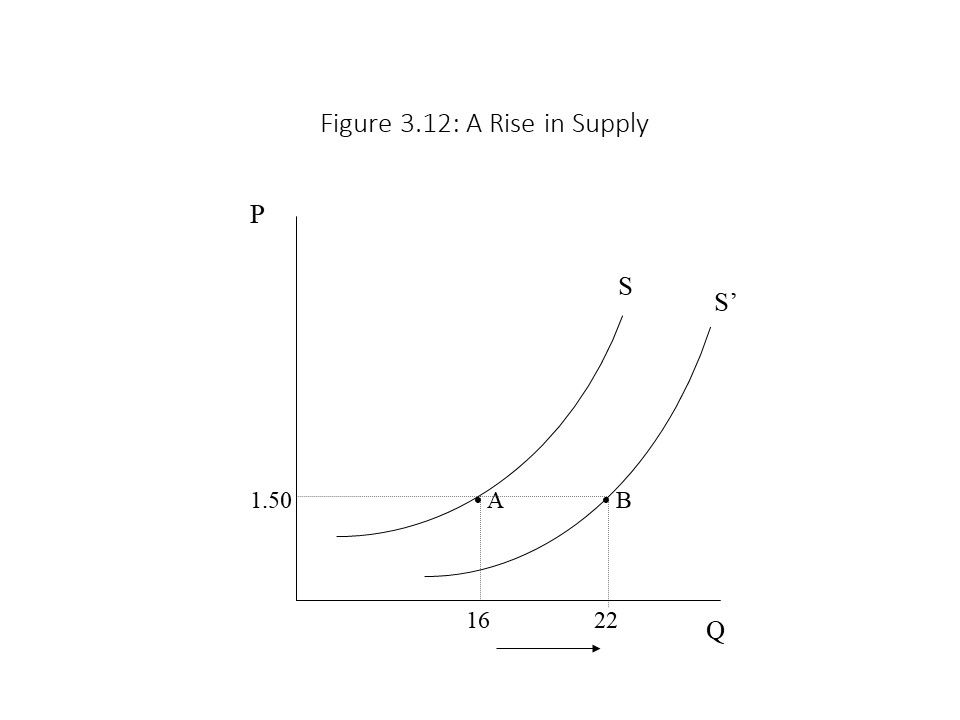 The quantity supplied of apples at a price of $1.50/lb. rises from 16 lbs. per month to 22 lbs. per month. Similar increases in the quantity supplied occur at every possible price. As a result, the entire supply curve shifts to the right. Neoclassical economists refer to such a shift as an increase in supply (as opposed to an increase in quantity supplied). By late fall, we might expect the quantity supplied of apples to fall at every price and the supply curve might shift to the left, back to its original position. Such a shift is referred to as a decrease in supply.
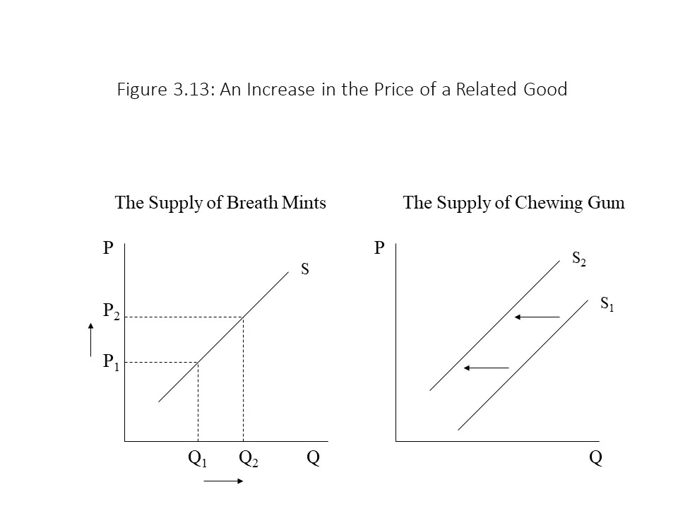 Prices of related goods:
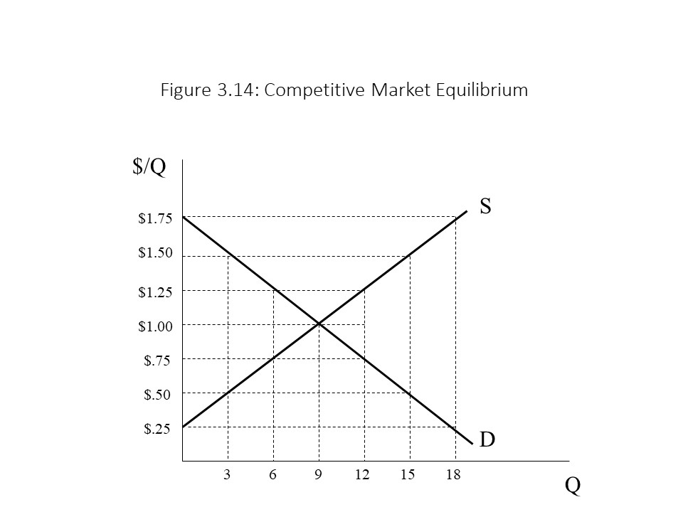 To understand how the equilibrium price and quantity exchanged come about in this market, it is best to begin at a price that is not the equilibrium price. For example, suppose the price begins at $1.75 per unit. In that case, the quantity demanded is 0 units, but the quantity supplied is 18 units. Because sellers wish to sell 18 more units at this high price than buyers wish to buy, we say that an excess supply, or a surplus, of the good exists. Due to the surplus, sellers will feel pressure to cut price. Suppose that sellers cut the price to $1.50 per unit. As the price falls, the quantity demanded rises to 3 units due to the law of demand. Similarly, the quantity supplied falls to 15 units due to the law of supply. The result is a smaller surplus of 12 units (= 15 units – 3 units). The sellers will continue to feel pressure to cut price as long as a surplus exists. The reader should try to determine what the quantity demanded, the quantity supplied, and the surplus are at a price of $1.25 per unit.
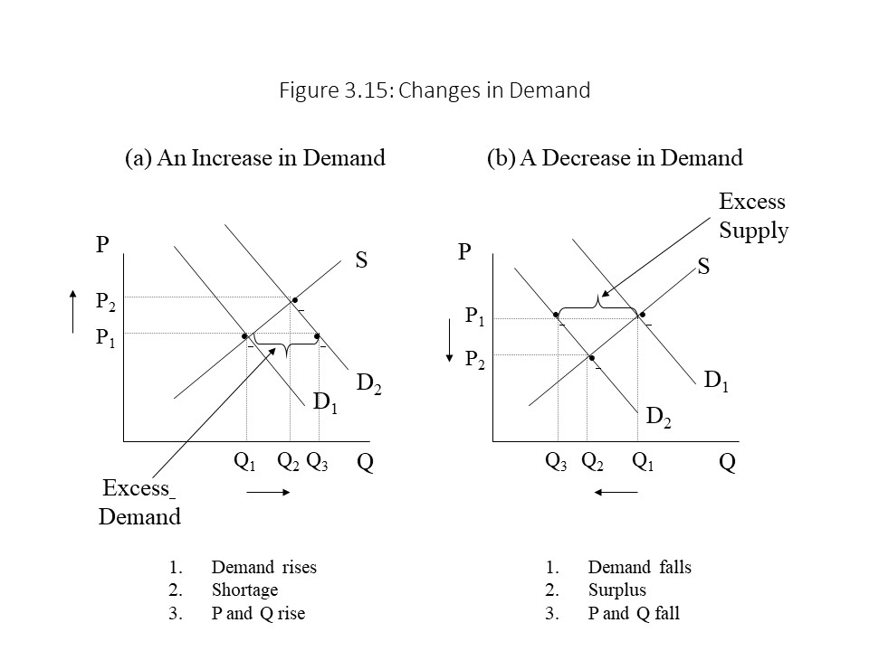
 To calculate the consumers’ surplus using this approach, it is only necessary to add up the shaded areas. We add the surplus of $0.50 on each of the units from 0 to 3, the surplus of $0.25 on each of the units from 3 to 6, and the surplus of $0.00 on the units from 6 to 9.
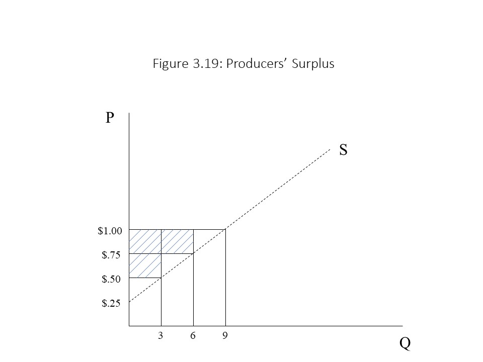 To calculate the producers’ surplus using this approach, it is only necessary to add up the shaded areas. We add the surplus of $0.50 on each of the units from 0 to 3, the surplus of $0.25 on each of the units from 3 to 6, and the surplus of $0.00 on the units from 6 to 9.
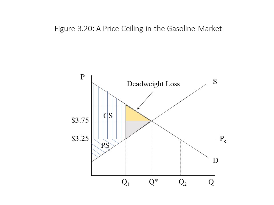 Because the price is prevented from rising above $3.25 per gallon, a shortage equal to Q2 – Q1 is the result. Furthermore, the shortage will persist indefinitely unless something else changes. The efficiency implications of the price ceiling are of even greater interest. Because only Q1 units of output are supplied at the low price, the consumers’ surplus and producers’ surplus on units Q* – Q1 are simply lost. This loss of surplus is referred to as deadweight loss. Therefore, any price set below the equilibrium price will reduce the total surplus realized in the market.
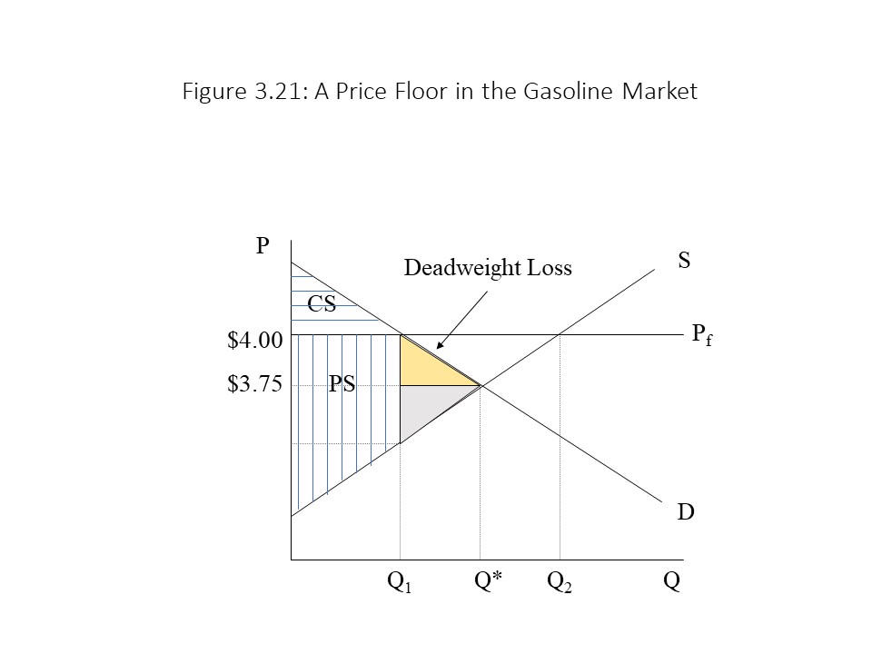 Because the price is prevented from falling below $4.00 per gallon, an excess supply equal to Q2 – Q1 is the result. Furthermore, the excess supply will persist indefinitely unless something else changes. The efficiency implications of the price floor are of great interest just as in the case of the price ceiling. Because only Q1 units of output are demanded at the high price, the consumers’ surplus and producers’ surplus on units Q* – Q1 are simply lost. As in the case of the price ceiling, deadweight loss is the result. Therefore, any price set above the equilibrium price will reduce the total surplus realized in the market.
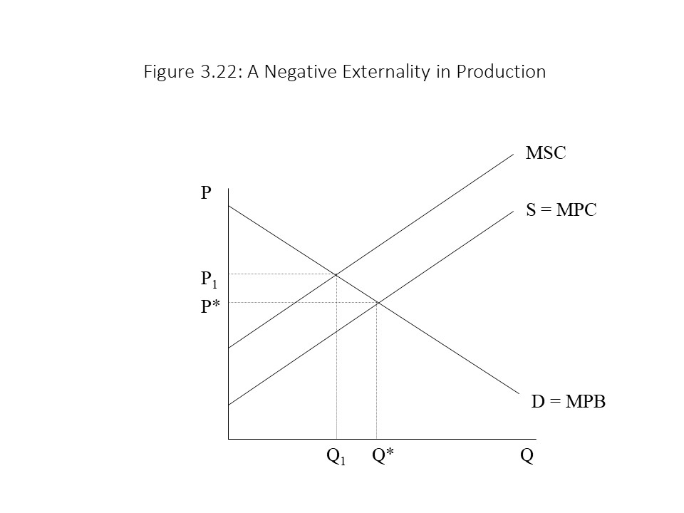
 In Figure 3.23, the market clears at P* and Q*. The efficient outcome, however, occurs where MSB intersects MPC at P1 and Q1. Because the efficient outcome occurs at a higher price and a higher quantity, the implication is that the good is under-priced and under-produced in a competitive market. The case might be made that a subsidy per unit given to consumers can be used to increase demand and bring it into line with MSB. Of course, it is difficult to know just how much of a tax or subsidy to impose in these cases of market failure. An error might lead to an even greater inefficiency than the one resulting in the case of competitive equilibrium.