Define the neoclassical concept of price elasticity of demand and explain its importance
Calculate and interpret the price elasticity of demand
Learn how and when to use the arc elasticity formula and the point elasticity formula
Identify key determinants of the price elasticity of demand
Explain the relationship between the price elasticity of demand and sales revenue
Define, calculate, and interpret other key measures of elasticity
The Need for a Measure of Consumer Responsiveness
In Chapter 3, we spent a great deal of time discussing the law of demand, which states that, other things equal, as the price of a good declines, the quantity demanded rises, and vice versa. In this chapter, we are interested in more than the direction of the change in quantity demanded when the price changes. That is, we wish to know the magnitude of the change in quantity demanded when the price changes. As a result, we require a measure of the change in quantity demanded when the price changes by some amount. This measure of the responsiveness of the consumer to a change in price is known to neoclassical economists as the price elasticity of demand.
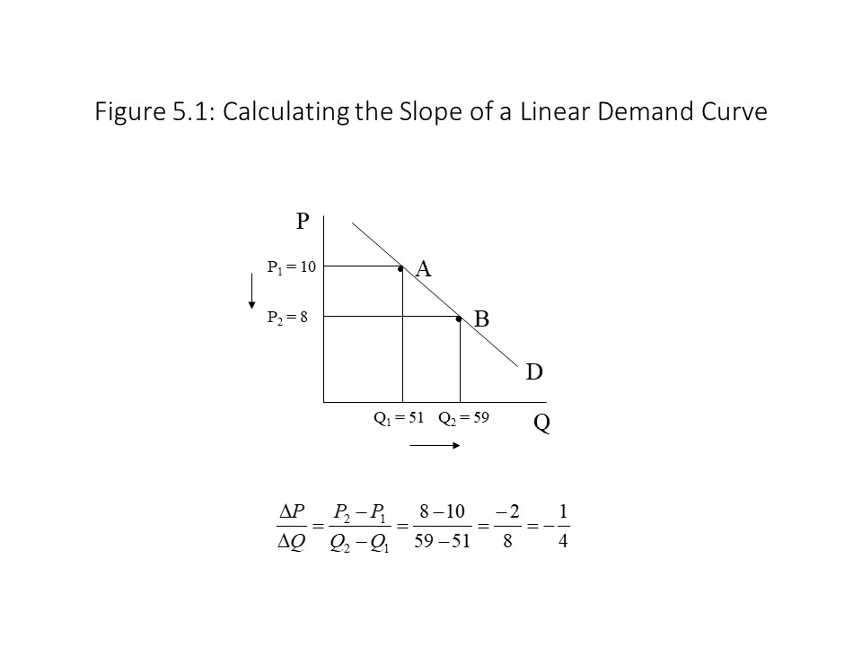
The reader may wonder why neoclassical economists require this special measure of consumer responsiveness to a price change. After all, the slope of the demand curve tells us the change in quantity demanded for a specific change in the price of the good. Figure 5.1 illustrates how to calculate the slope of a linear demand curve.
In Figure 5.1, the price of the good declines from $10 per unit to $8 per unit and the quantity demanded rises from 51 units to 59 units of the good. The movement from point A to point B reveals that the slope is equal to -1/4. The slope appears to provide us with a measure of the responsiveness of the consumer to a price change. A serious problem exists, however, with this measure of consumer responsiveness. Specifically, it is not a unit-free measure of consumer responsiveness, and therefore, it does not permit comparisons of consumer responsiveness across different markets. To better grasp this point, consider Figure 5.2.Figure 5.2, the slopes of the two demand curves are both equal to -1/2, suggesting that the consumers are equally responsive to price changes in the two markets. The problem, however, is that we are comparing apples and oranges, or in this case, textbooks and automobiles. In other words, the slope of the demand curve is not a unit-free measure of consumer responsiveness. More generally, we might ask in which units the slope is measured. The price of a good is measured in dollars per unit of the good ($/Q). The slope then, which is calculated as ∆P/∆Q, must be measured in terms of ($/Q)/Q or $/Q2.[1] Clearly, this measure is not unit-free and will not allow direct comparisons of consumer responsiveness across markets.
Calculating and Interpreting the Price Elasticity of Demand
The price elasticity of demand is a measure that avoids the shortcomings of the slope of the demand curve as a measure of consumer responsiveness. It is calculated in the following way, where ED refers to the price elasticity of demand:
For example, when the price of a good rises by 6% and the quantity demanded of the good falls by 12%, then the price elasticity of demand is equal to -2 as shown in the following calculation:
The careful reader will notice two important differences between this measure and the slope of the demand curve. First, the price elasticity of demand places Q in the numerator and P in the denominator, which suggests that this measure will be inversely related to slope. Second, the price elasticity of demand includes percentage changes as opposed to absolute changes in P and Q.
The next question we must ask, however, is whether this measure of consumer responsiveness is unit-free. Only then will it be possible to make comparisons of consumer responsiveness across markets. It turns out that it is unit-free. Consider, for example, a child that begins the month weighing 100 lbs. At the end of the month, the child weighs 105 lbs. Because the child’s original weight (W) is 100 lbs. and the change in the child’s weight (∆W) is 5 lbs., the percentage change in the child’s weight (∆W/W) is 5 lbs./100 lbs. or 5%. The reader can easily see that the units cancel out in this calculation, leaving us with a pure or unit-free number. It is the same way with all calculations involving percentages. In the case of the price elasticity of demand, we can rewrite the formula in the following way:
The reader should note that cancellation of the units in the numerator and denominator of this fraction leads to the calculation of a unit-free measure of consumer responsiveness.
If we return to the example in which the price elasticity of demand was calculated to be -2, it is natural to wonder why the result has included a negative sign. This result should come as no surprise because the law of demand states that price and quantity demanded are inversely related, other things held constant. In fact, we should almost always expect a negative sign when we calculate the price elasticity of demand. For this reason, neoclassical economists typically omit the negative sign when referring to the price elasticity of demand and instead refer to its absolute value. A neoclassical economist would state then that the price elasticity of demand is 2 even though she really means -2. Our formula for the price elasticity of demand can be modified as follows, and the previous calculation would be carried out as shown:
The absolute value of the price elasticity of demand is used then as a kind of shorthand. It is useful as well for another reason. When the absolute value of the price elasticity of demand is equal to 2, it can be interpreted to mean that a 1% rise in price causes a 2% reduction in quantity demanded, other things equal. If the absolute value is equal to 3, then a 1% rise in the price causes a 3% reduction in quantity demanded. In the latter case, we observe a larger response from consumers given a 1% rise in price. When consumers are more responsive to a price change, it is said that demand is more elastic. Because we are referring to the absolute value, the larger the number is, the more elastic the demand will be. If we were using the negative values, then we would be forced into the less natural position of claiming that the lower the value, the greater the elasticity of demand.
More generally, the price elasticity of demand may take on any value from zero to positive infinity (in absolute value terms). Depending on the specific value, different language is used to refer to the elasticity of demand. Below are the phrases used for each possible range of values. The symbol “” indicates that the two statements are logically equivalent.
It has already been emphasized that a larger price elasticity of demand implies greater responsiveness on the part of consumers. Nevertheless, more must be said to explain why a value of 1 is so important to the interpretation of this value. To understand the reason, we return to the definition of the price elasticity of demand and observe the following:
That is, when demand is unit elastic, a 5% rise in price leads to a 5% reduction in quantity demanded. The consumers, in other words, respond by an equal percentage amount to a price change. For this reason, the value of 1 is important for the purposes of interpreting the price elasticity of demand.
When the price elasticity of demand exceeds 1, we have the following:
This result indicates that demand is elastic whenever the consumers respond by a greater percentage amount than the price change (in absolute value terms).
When the price elasticity of demand is less than one, we have the following:
This result indicates that demand is inelastic whenever the consumers respond by a smaller percentage amount than the price change (in absolute value terms).
When the price elasticity of demand is equal to 0, we have the following:
This result indicates that demand is perfectly inelastic whenever the consumers do not respond at all to a given percentage change in the price of the good.
Finally, when the price elasticity of demand is equal to ∞, we have the following:
Division by zero causes the fraction to be undefined. In this case, however, we can imagine a very tiny percentage price change such that it approaches 0 and the entire fraction, therefore, approaches infinite. In other words, even for the smallest (nearly zero) change in price, we obtain an opposite change in quantity demanded. That is consumers are perfectly responsive to any price change at all, and demand is said to be perfectly elastic.
Notice that with this measure we can now compare the responsiveness of orange consumers and apple consumers if we know the price elasticity of demand for each. If the price elasticity of demand for oranges is 2 and the price elasticity of demand for apples is 3, then we conclude that apple consumers are relatively more responsive than orange consumers to price changes. In a sense, we are free to compare apples and oranges, which was not possible when we only knew the slopes of the demand curves.
The Arc Elasticity and Point Elasticity Formulas
When we know the percentage changes in price and quantity demanded, it is very easy to calculate the price elasticity of demand. We simply use the definition of the price elasticity of demand that was provided in the previous section. At times, however, we might find ourselves only knowing the absolute changes in price and quantity demanded. Without direct knowledge of the percentage changes in price and quantity demanded, we must find some way of obtaining this information from the information we do have. For example, consider the graph in Figure 5.3.
In this case, we know that the price of the good rises from $4 per unit to $5 per unit and that the quantity demanded subsequently falls from 22 units to 18 units. That is, we know only the absolute changes in price and quantity demanded. To convert our formula for the price elasticity of demand from one that uses percentage changes to one that uses absolute changes, we need to return to our initial definition and make the conversion as follows:
This formula appears to solve our problem because we can now use absolute quantities and prices to carry out a calculation of the price elasticity of demand. Unfortunately, the formula has one major defect. The problem with this formula is that it is not immediately clear which Q and P should be used in the denominator of each fraction. When neoclassical economists first considered this problem, they decided that it would be completely arbitrary to use Q1 and P1 as opposed to Q2 and P2. The issue is important because the calculation is different depending on the choice that is made. As a result, they concluded that it made the most sense to use the average quantity demanded and the average price when carrying out the calculation. As a result, the formula changes to the following:
If we write the arc elasticity formula in terms of its absolute value and carry out the calculation using the information provided in Figure 5.3, then we obtain the following:
The reader should note that the average quantity demanded of 20 units and the average price of $4.50 per unit (= 9/2) is in Figure 5.3 at the midpoint between the two points on the demand curve that we have been considering. Another point to notice is that it is possible to conclude that demand is inelastic in this case because 9/10 is less than 1. Therefore, consumers are relatively unresponsive to price changes, at least between these two points on the demand curve.
The arc elasticity formula works well when we wish to calculate the price elasticity of demand between two points on the demand curve as in Figure 5.3. At other times, we might wish to calculate the price elasticity of demand at a single point on the demand curve. It might seem like an impossible task given that our initial formula depends upon changes in price and quantity demanded. It is still possible, however, to calculate the price elasticity of demand in such situations if we know that the demand curve is linear and we can determine the slope. For example, if we have the information given in Figure 5.4, then we can calculate the price elasticity of demand at a specific point.
To understand how this information can be used to calculate the price elasticity of demand, we can convert our original formula in the following way:
The final expression is the point elasticity formula. It is now possible to calculate the price elasticity of demand for a given P and Q on the demand curve. The reader should also note that ∆P/∆Q represents the slope of a linear demand curve. If we use the information in Figure 5.4 to calculate the absolute value of the price elasticity of demand using the point elasticity formula, then we obtain the following result:
In this case, the price elasticity of demand is greater than 1. Therefore, we conclude that demand is elastic at this point on the demand curve. That is, consumers are relatively responsive to the price change.
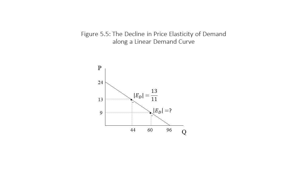
The reader might expect the price elasticity of demand to be the same at every point on this linear demand curve. After all, the slope is constant at every point on the demand curve. This conclusion is incorrect, however, as can be shown by calculating the price elasticity of demand at another point on the demand curve. For example, we might calculate the price elasticity of demand at a second point on the linear demand curve we just considered as shown in Figure 5.5.
If we calculate the price elasticity of demand when the price is equal to $9 per unit and the quantity demanded is equal to 60 units, then we obtain the following result:
In this case, we conclude that demand is inelastic because the price elasticity of demand is less than 1. It should also be noted that the slope of -1/4 remains the same in this calculation. The only change in this calculation compared with the calculation when the price is equal to $13 per unit is the specific P and Q that we use as we move down the demand curve. What we observe is that the price elasticity of demand declines as we move down the linear demand curve. This general result can be explained intuitively. That is, consumers are less responsive to price changes at lower prices than at higher prices. In other words, a 5% price reduction when the price is very high has a greater impact on the consumer’s quantity demanded than a 5% price reduction when the price is very low.
We thus obtain a major result: the price elasticity of demand falls as the price falls along a linear demand curve.
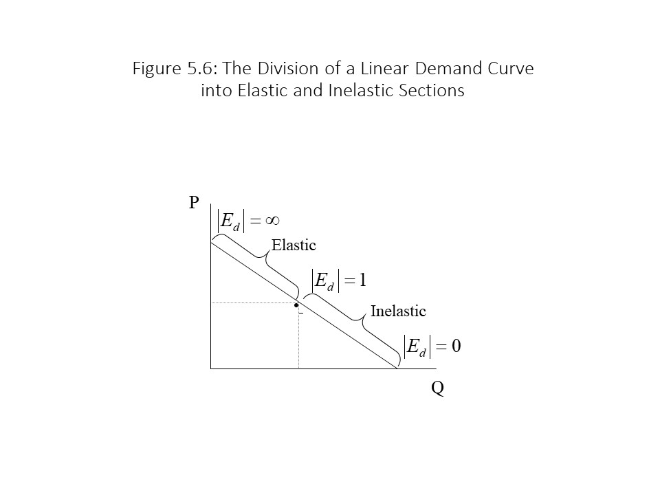
The point elasticity formula can also be used to divide a linear demand curve into elastic and inelastic sections as shown in Figure 5.6.
For example, we can calculate the price elasticity of demand where the demand curve intersects the vertical axis as follows:
In this case, for any price and slope, the price elasticity of demand will be (or will approach) infinity.
We can also calculate the price elasticity of demand where the demand curve intersects the horizontal axis as follows:
In this case, for any Q and slope, the price elasticity of demand will be zero.
Furthermore, the point elasticity formula indicates that as the price falls and the quantity demanded rises along a linear demand curve, the ratio of P to Q (that is, P/Q) will decline causing the price elasticity of demand to fall. Therefore, the price elasticity of demand falls continuously from its highest value of infinity to its lowest value of zero as we move down along the linear demand curve. Due to the continuous decline in the price elasticity of demand, at some point, the price elasticity of demand will equal 1. That is, demand will be unit elastic. This point marks the separation between the elastic portion of the demand curve (where |ED|>1) and the inelastic portion of the demand curve (where |ED|<1).
Cases of Extreme Elasticity
In certain situations, demand may become perfectly elastic or perfectly inelastic at every price on the demand curve. These situations are unusual but theoretically possible. For example, a consumer might become perfectly unresponsive to price increases if she is in desperate need of a life-saving medication. No matter how high the price rises, the consumer will pay the price and not reduce her quantity demanded. Of course, even this case has limits because the consumer will eventually become unable to make the purchase even if she is still willing to do so. (The reader will recall that both ability and willingness to pay are required for the demand for a product to exist.) Nevertheless, in this case, the demand curve becomes perfectly vertical as shown in Figure 5.7.
As the reader can see, even when the price rises from P1 to P2, the quantity demanded remains unchanged at Q1. Because the slope of the demand curve is infinite in this case, the use of the point elasticity formula yields the following result:
It is clear then that demand is perfectly inelastic when the slope of the demand curve is infinite. It should also be clear that the slope of the demand curve and the price elasticity of demand are inversely related.
A second extreme case arises when consumers become perfectly responsive to price changes. That is, the smallest rise in price may lead consumers to reduce their quantity demanded to 0. Alternatively, the smallest reduction in price might lead consumers to increase their quantity demanded to infinity (or a very large quantity, at least!). This might occur when a consumer knows that a perfectly good substitute product is available at the same price. As soon as the price of the product the consumer is buying rises at all, he switches immediately to the other product and his quantity demanded of the first product falls to zero. This situation is depicted in Figure 5.8 as a horizontal demand curve.
As the reader can see, for any price above P1 the quantity demanded will equal zero and for any price below P1 the quantity demanded will soar to infinity. Because the slope of the demand curve is zero in this case, the price elasticity of demand can be calculated as follows:
Demand is perfectly elastic then when the slope of the demand curve is equal to 0, and we again see that the slope of the demand curve and the price elasticity of demand are inversely related.
Key Determinants of the Price Elasticity of Demand
At this point, we have considered several ways to calculate the price elasticity of demand, but it is also necessary to consider the factors that cause the demand for a product to be more (or less) elastic. The key determinants of the price elasticity of demand include the following:
The nature of the good: Is it a luxury or a necessity?
If the good is a luxury item then consumers can do without it. If the price rises, consumers will be highly responsive to the price change. Similarly, if the price falls, consumers will be eager to enter this market. On the other hand, if the good is a necessity, like the life-saving medication described above, then consumers will not be able to reduce their purchases very much when the price rises. Alternatively, if the price falls, consumers will not expand their purchases much because they were already purchasing the amount required before the price fell. In general, the price elasticity of demand for luxuries tends to be greater than the price elasticity of demand for necessities, other things the same.
The budget share devoted to the purchase of the good
If consumers spend a large percentage or share of their budgets on a good, then the demand for the good tends to be more elastic, other things the same. The reason is obvious. Consumers will feel a greater pinch from a rise in the price of an automobile than they will feel from the rise in the price of chewing gum. Consumers of automobiles are, therefore, more responsive to price changes than consumers of chewing gum.
The time spanduring which the good is purchased
The reader should recall from Chapter 3 that the quantity demanded of a product is a flow variable. That is, it is defined per period, such as a day, a week, a month, or a year. If the period is very short, such as a day, then the demand for a good tends to be inelastic, other things the same. For example, when the price of gasoline rises sharply, consumers are often slow to reduce their purchases. Consumers still need to drive to work and to school. Over long periods, however, consumers can begin to seek out substitute forms of transportation. For example, they can carpool, ride the bus, or ride a bike. As a result, consumers are more responsive to price changes over longer periods than over shorter periods. In general, the demand for a good is more elastic in the long run than in the short run, other things the same.
The existence of substitutes
Finally, if many close substitutes for a good exist, then consumers tend to be more responsive to price changes. For example, if the price of apple juice rises sharply, consumers can substitute towards grape juice. As a result, the quantity demanded of apple juice drops sharply. On the other hand, if the price of juice in general rises, then consumers can substitute towards milk or soda, but these alternatives are not very good substitutes for juice. As a result, the demand for juice is much more inelastic than the demand for apple juice. In general, when more close substitutes for a good exist, demand tends to be more elastic, other things the same.
Below are a few examples of demand elasticities in different industries.[2]
Example 1: The price elasticity of demand for restaurant meals has been estimated to be 2.27.
Example 2: The short run price elasticity of demand for gasoline has been estimated to be 0.3.
Example 3: The price elasticity of demand for premium white pan bread has been estimated at 1.01.
The high demand elasticity of restaurant meals can be attributed to the perception among many consumers that they are luxury goods. The low demand elasticity for gasoline can be attributed to the short period and the perception that gasoline is a necessity. Finally, the relatively elastic demand for premium white pan bread may be attributed to the existence of many close substitutes.
The Relationship between the Price Elasticity of Demand and Sales Revenue
When a firm sells a particular product, its sales revenue, or total monetary receipts, depends on two important variables: the price per unit and the number of units sold. In other words, a firm’s revenue depends on price and quantity demanded. Specifically, we can calculate a firm’s revenue by multiplying the product price by the quantity demanded. If we consider a linear demand curve, like the one shown in Figure 5.9, then it is possible to represent total revenue (TR) as the product of P and Q, or as the area of the box under the demand curve.
In this case, the total revenue is $50 or $5 per unit times 10 units.
A manager of a firm now faces a difficult task. If the manager aims to increase revenue, it might seem logical to raise the price of the good. The problem is that the quantity demanded will fall as the price rises, according to the law of demand. Therefore, we observe two conflicting effects on total revenue when the price changes, as shown below, leaving the overall effect an open question.
The manager must ask which factor has the greater impact on revenue. In other words, what is the net effect of a change in price?
The answer to this question, it turns out, depends on the price elasticity of demand. Let’s consider a price reduction that leads to a rise in quantity demanded. Although we do not provide a rigorous proof of this result, we can provide an intuitive explanation for these changes. If the price falls by the same percentage as the rise in quantity demanded, then the net effect on total revenue is zero. On the other hand, if the price falls by a greater percentage than the rise in quantity demanded, then the net effect on total revenue is negative.[3] Finally, if the price falls by a smaller percentage than the rise in quantity demanded, then the net effect on total revenue is positive. These results and the implications for demand elasticity are shown below with larger arrows indicating larger percentage changes.[4]
Because we identified the elastic and inelastic portions of a linear demand curve earlier in this chapter, we can now use that information to determine the shape of the total revenue curve. Figure 5.10 reveals that as the price falls from its peak, total revenue rises because demand is elastic. Once we reach the point where demand is unit elastic, total revenue does not change (the meaning of the overbar above TR in the unit elastic case shown above). Finally, if price falls far enough, then total revenue declines because demand is inelastic.
The reader can see that when the price elasticity of demand is infinite, total revenue is equal to 0. Although the price is high, the quantity demanded is zero. Similarly, when the price is set at 0, total revenue is equal to 0 even though the quantity demanded is high at Q2. In between these two extremes, the total revenue rises and then falls as the price declines. Because total revenue rises prior to the point of unit elasticity and falls after the point of unit elasticity, it follows that total revenue reaches its peak at the point of unit elasticity. Although total revenue reaches its maximum at Q1, the reader should not assume that this level of output is the optimal choice for the firm. The firm must also consider production cost, which is a concept that is discussed at great length in Chapter 7.
Other Measures of Elasticity: Supply, Cross-Price, and Income
The price elasticity of demand is a widely used concept among neoclassical economists, in part because of its connection to sales revenue. Several other elasticity concepts are also useful, namely the price elasticity of supply, the cross-price elasticity of demand, and the income elasticity of demand. This section only provides a brief overview of these concepts.
The Price Elasticity of Supply
Just as consumers are responsive to changes in price, so are sellers. To measure the responsiveness of sellers to price changes, neoclassical economists use the price elasticity of supply defined below:
The formula for the price elasticity of supply (ES) measures the percentage change in the quantity supplied for a given percentage change in price. For example, if the price of a product increases by 8% and the quantity supplied rises by 24%, then the price elasticity of supply equals 3. It should be noted that it is not necessary to calculate the absolute value of the price elasticity of supply as we did earlier with the price elasticity of demand. The reason is that the price elasticity of supply will virtually always be a positive number due to the law of supply. That is, price increases will lead to increases in quantity supplied and price reductions will lead to reductions in quantity supplied.
When the price elasticity of supply equals 3, it may be interpreted to mean that a 1% rise in price leads to a 3% rise in quantity supplied, or a 1% reduction in price leads to a 3% reduction in quantity supplied. The interpretations of price elasticity of supply are also like the interpretations of the price elasticity of demand. For example, if the price elasticity of supply equals 1, then supply is unit elastic. If it is greater than 1, then supply is elastic. If it is less than 1, then supply is inelastic. If it is infinite, then supply is perfectly elastic. If it is equal to 0, then supply is perfectly inelastic.
The primary determinant of the price elasticity of supply is the time frame. If the price of apples rises in a very short period such as a month, for example, then producers of apples cannot expand production very quickly. They can hire more workers to pick more apples, but they cannot grow more apples in a month’s time. The price elasticity of supply in the short run tends to be very low, as a result. Over a longer period, it may be possible to purchase additional orchards or even to grow more trees. Supply then becomes much more elastic. That is, producers can expand production as the price rises over long time periods. Figure 5.11 shows an inelastic short run supply curve and a much more elastic long run supply curve.
The Cross-Price Elasticity of Demand
The cross-price elasticity of demand (or simply, cross elasticity) allows us to measure the percentage change in the quantity demanded of a product for a given percentage change in the price of a different product. For example, the cross elasticity of demand between goods A and B can be written as follows:
If the price of good B rises by 4% and the quantity demanded of good A rises by 2%, then the cross elasticity is equal to +1/2. In this case, the sign is important. The fact that the consumer purchases more of good A when the price of good B rises indicates that the consumer considers good A to be a substitute for good B. Similarly, if the price of peanut butter rises by 6% and the quantity demanded of jelly falls by 2%, then the cross elasticity is -1/3. Because the consumer reduces purchases of jelly when the price peanut butter rises, it suggests that the goods are often consumed together. In other words, the two goods are complements. Finally, the two goods are regarded as unrelatedgoods if the quantity demanded does not change at all when the price of the other good changes. That is:
The reader should notice that a positive value for the cross elasticity may be obtained either with a +/+ or a -/-. Similarly, a negative value for the cross elasticity may be obtained either with a +/- or a -/+.
The cross elasticity has an important application in antitrust law. Consider two firms that are trying to initiate a merger. If the merger reduces competition and leads to higher prices, then the merger will harm consumers. Antitrust laws are in place to prevent such mergers, but it is not always obvious whether two goods are substitutes for one another. If they are, then the merger will reduce competition. As a result, the U.S. Justice Department, which enforces the nation’s antitrust laws, may ask an expert to testify in antitrust cases that two goods have a positive cross elasticity. Such evidence supports the claim that the goods are substitutes and that a merger of the two firms will harm American consumers.
The Income Elasticity of Demand
One final elasticity measure that we will consider is the income elasticity of demand. This elasticity concept measures the responsiveness of consumers to a change in income. That is, it measures the percentage change in the quantity demanded of a product given a percentage change in income (Y). It can be written as follows:
For example, if a 3% rise in income leads to a 12% rise in quantity demanded, then the income elasticity of demand is equal to +4. The sign of the income elasticity of demand is also important. The positive sign in this case indicates a positive relationship between income and quantity demanded. In Chapter 3, we explained that such goods are called normal goods. Alternatively, if a 3% rise in income leads to a 6% drop in quantity demanded, then the income elasticity of demand is -2. Such goods are called inferior goods because a negative relationship exists between income and quantity demanded. Finally, if the quantity demanded does not change at all when income changes, then the income elasticity of demand is equal to 0. Such goods are said to be neutral with respect to income. That is:
The reader should note that a positive income elasticity of demand may be obtained with either a +/+ or a -/-. The reader should also note that a negative income elasticity of demand may be obtained with either a +/- or a -/+.
Do Marxian Economists Use Elasticity Measures?
Before concluding this chapter, it is worth noting that Marxian economists do not make much use of elasticity measures. One reason is that the price elasticities of supply and demand are measures that relate to market supply and demand curves. For neoclassical economists, supply and demand provide the best explanation of market prices. For Marxian economists, supply and demand influence market prices, but these laws are subordinate to the law of value. That is, socially necessary abstract labor time governs commodity values and so it is the law of value that receives the attention of Marxian economists. Similarly, Marxian economists are interested in the class dynamics of capitalist societies. How consumers respond, and to what extent they respond, to price changes is not a major concern of Marxian economists. A second reason is that the two primary measures that Marxian economists use to draw comparisons across industries are unit-free measures. Recall that the rate of surplus value and the rate of profit measure the degree of exploitation of labor-power and the rate of self-expansion of capital in different industries, respectively. Both measures are already expressed in percentage terms and so direct comparisons across industries are possible. In Chapter 8, we will see that such comparisons across industries play an important role in the Marxian theory of industrial competition.
Business executives are very aware of the issue of consumer responsiveness to price changes. For example, the Chief Executive of Hershey Co., Michele Buck, explained in an interview that Hershey recently increased the prices of its products but that she does not expect people to reduce their candy purchases in response to the higher prices. In other words, Ms. Buck believes that the demand for Hershey products is relatively inelastic. She anticipates a rise in sales as Hershey introduces new “stand-up pouches” for its candy bags, which “look more appealing on shelves.” If sales revenues rise even as prices are increased, then that result would certainly be consistent with Ms. Buck’s contention that the demand for Hershey’s candy is relatively inelastic (i.e., less than one in absolute value). Innovation is used to justify the price increases for food products with inelastic demands. In addition to Hershey’s new packaging, it also is introducing a “thinner Reese’s peanut butter cup … that it hopes will appeal to calorie-conscious Americans.” Gasparro likens this new product to Oreo Thins, which Mondelez International, Inc. introduced in 2015. Because of these kinds of innovations, Hershey managed to increase total sales by 2.5% to $1.99 billion in the fourth quarter of 2018. Although a rise in total revenue does not necessarily correspond to an increase in total profit, in this case, profits did rise in the fourth quarter by 24%. The implication is that the price increases are not only boosting sales revenue, they are part of an overall profit-maximizing strategy as well.
Summary of Key Points
The price elasticity of demand measures the responsiveness of consumers to price changes.
Unlike the slope of the demand curve, the price elasticity of demand is a unit-free measure.
A larger absolute value of the price elasticity of demand implies that demand is more elastic.
The arc elasticity formula is used to calculate price elasticity of demand when moving between two points on a demand curve; the point elasticity formula is used to calculate the price elasticity of demand at a single point on the demand curve.
The price elasticity of demand depends on the nature of the good, the time span, the budget share, and the existence of substitutes.
Whether total revenue rises, falls, or remains the same when price changes, depends on whether demand is elastic, inelastic, or unit elastic.
The price elasticity of supply measures the responsiveness of sellers to price changes.
The cross-price elasticity of demand measures the responsiveness of consumers to a change in the price of a different good.
The income elasticity of demand measures the responsiveness of consumers to a change in their incomes.
We do not use the absolute value of supply elasticity, cross elasticity, and income elasticity because the signs of these values are highly significant.
List of Key Terms
Price elasticity of demand
Elastic
Unit elastic
Inelastic
Perfectly inelastic
Perfectly elastic
Arc elasticity
Point elasticity
Total revenue
Price elasticity of supply
Cross-price elasticity of demand
Substitutes
Complements
Unrelated goods
Income elasticity of demand
Normal goods
Inferior goods
Neutral goods
Problems for Review
Suppose the price of a good rises by 6% and the quantity demanded falls by 30%. What is the price elasticity of demand (in absolute value terms)? Also, interpret your answer.
Suppose the price of a good falls from $62 to $58 and the quantity demanded rises from 1,760 units to 1,910 units. Calculate the price elasticity of demand using the arc elasticity formula. Also, interpret your answer.
Suppose the price of a good is $45 and the quantity demanded is 500 units. If the slope of the linear demand curve is -3, then what is the price elasticity of demand, according to the point elasticity formula? Also, interpret your answer.
If the price of gasoline rises and the total revenue received by sellers decreases, then what can you conclude about the relationship between the percentage change in quantity demanded relative to the percentage change in price (in absolute value)? What can you conclude about the price elasticity of demand?
If the price of cereal rises by 2% and the quantity demanded of milk falls by 0.5%, then what is the cross elasticity between the two products? Also, interpret your answer. Is your interpretation consistent with your expectations?
If your income rises by 10% and your quantity demanded of used goods falls by 20%, then what is the income elasticity of demand? Interpret your answer. Is your answer consistent with your expectations?
I wish to acknowledge Prof. John Hoag for first emphasizing to me the units in which slope is measured. ↵
Recalling that the %∆xy ≈ %∆x+%∆y, we can write that %∆PQ ≈ %∆P+%∆Q. If revenue falls, then %∆P+%∆Q < 0, and %∆Q < -%∆P. In the case of a price decrease and an increase in quantity demanded, it follows that the percentage change in price exceeds the percentage change in quantity demanded (in absolute value terms). Hence, demand is inelastic. ↵
It is left to the reader to consider how to analyze the three cases when the price increases. ↵
Gasparro, Annie. The Wall Street Journal (Online); New York. 31 Jan. 2019. ↵


 In Figure 5.1, the price of the good declines from $10 per unit to $8 per unit and the quantity demanded rises from 51 units to 59 units of the good. The movement from point A to point B reveals that the slope is equal to -1/4. The slope appears to provide us with a measure of the responsiveness of the consumer to a price change. A serious problem exists, however, with this measure of consumer responsiveness. Specifically, it is not a unit-free measure of consumer responsiveness, and therefore, it does not permit comparisons of consumer responsiveness across different markets. To better grasp this point, consider Figure 5.2.
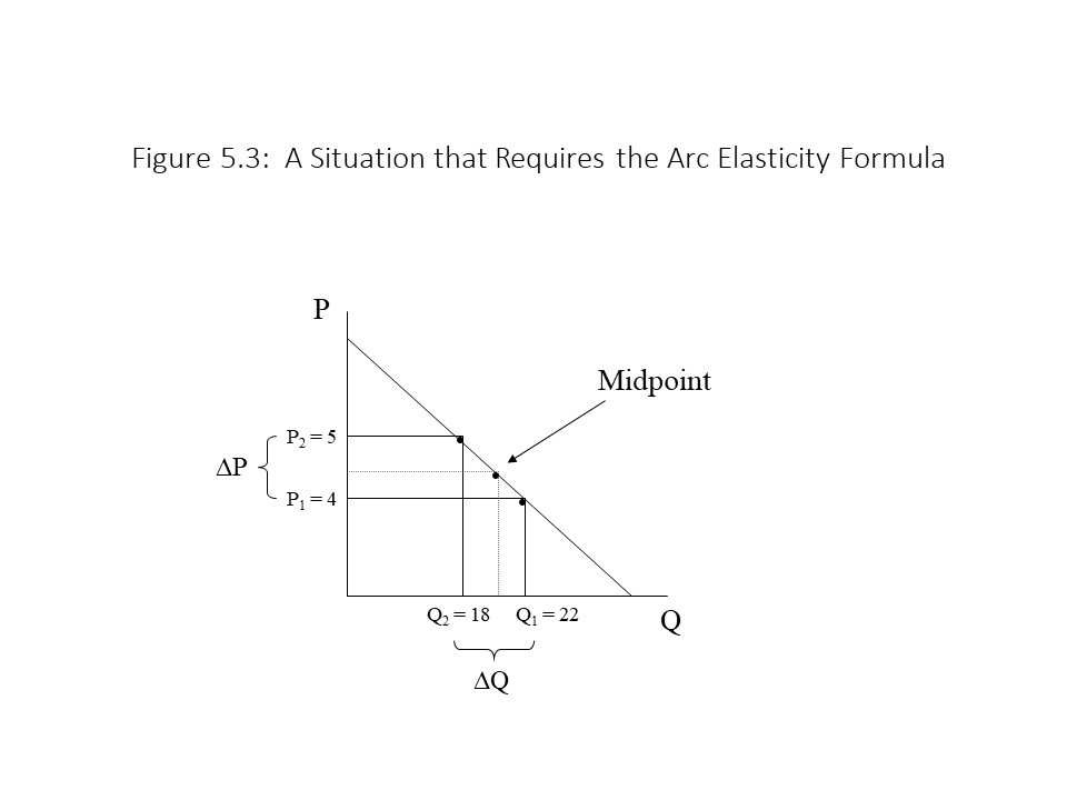 In this case, we know that the price of the good rises from $4 per unit to $5 per unit and that the quantity demanded subsequently falls from 22 units to 18 units. That is, we know only the absolute changes in price and quantity demanded. To convert our formula for the price elasticity of demand from one that uses percentage changes to one that uses absolute changes, we need to return to our initial definition and make the conversion as follows:
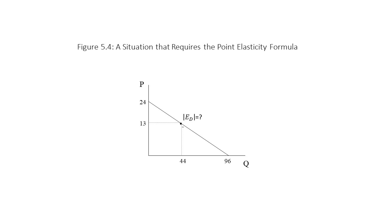
 For example, we can calculate the price elasticity of demand where the demand curve intersects the vertical axis as follows:
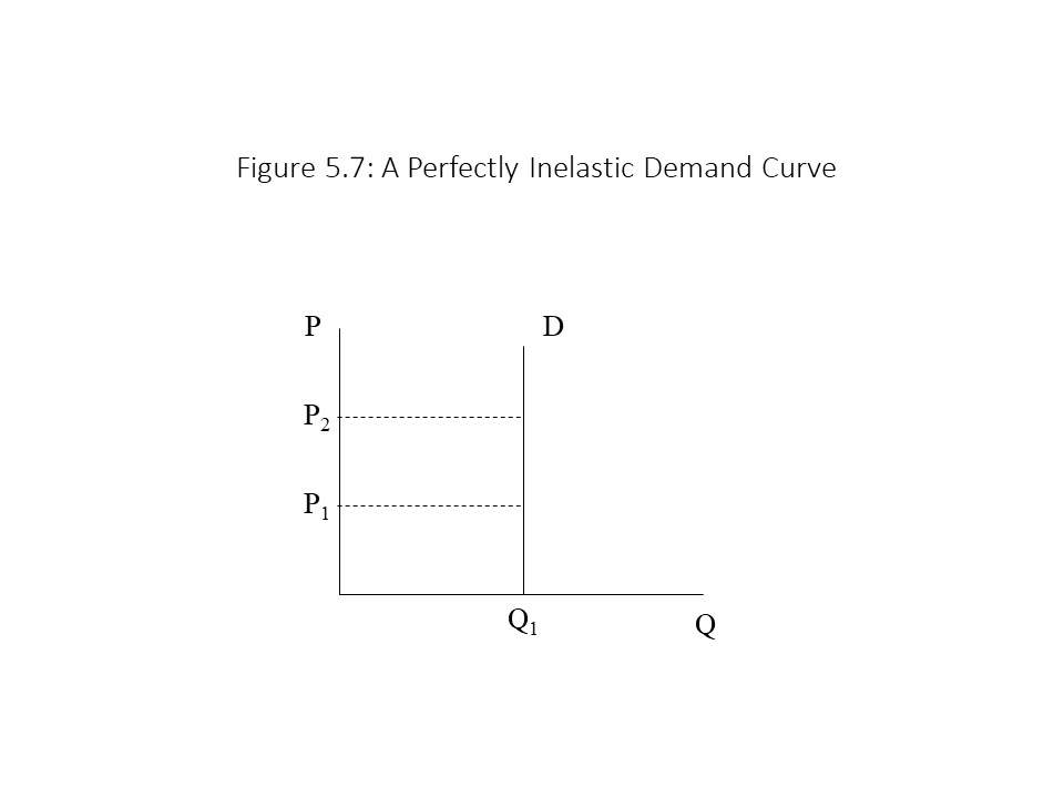 As the reader can see, even when the price rises from P1 to P2, the quantity demanded remains unchanged at Q1. Because the slope of the demand curve is infinite in this case, the use of the point elasticity formula yields the following result:
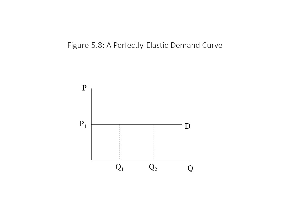 As the reader can see, for any price above P1 the quantity demanded will equal zero and for any price below P1 the quantity demanded will soar to infinity. Because the slope of the demand curve is zero in this case, the price elasticity of demand can be calculated as follows:
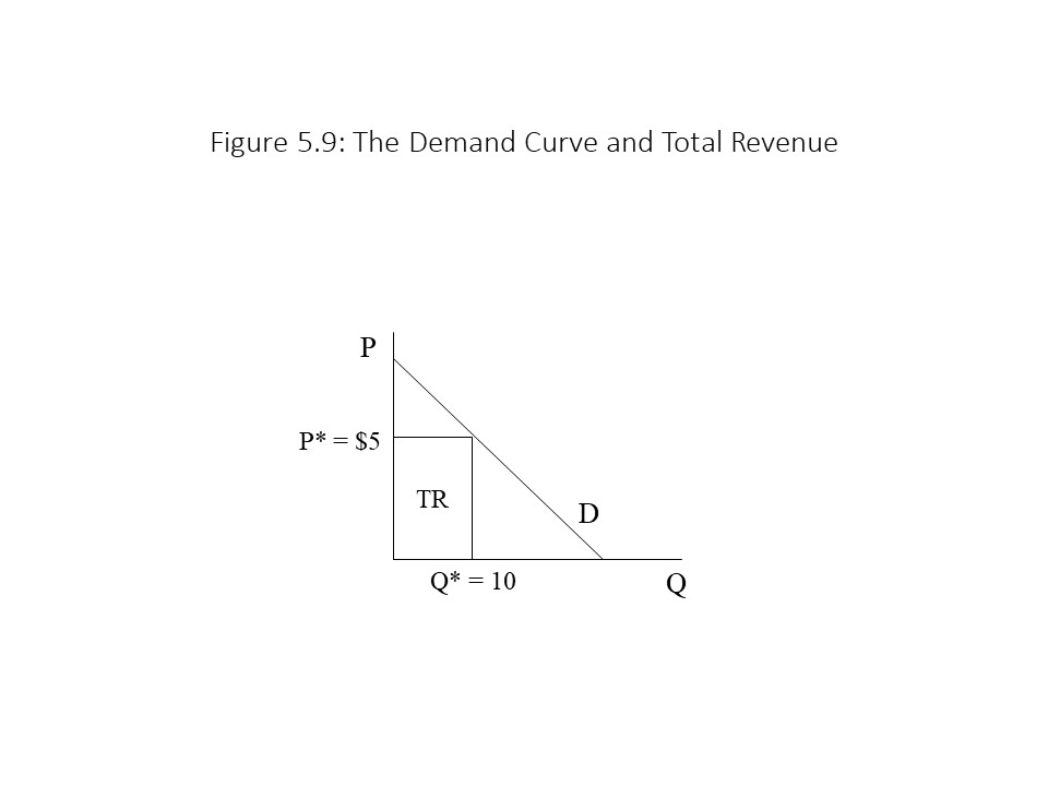 In this case, the total revenue is $50 or $5 per unit times 10 units.
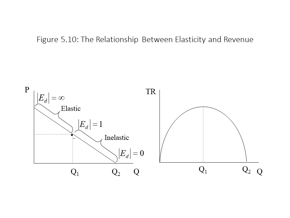 The reader can see that when the price elasticity of demand is infinite, total revenue is equal to 0. Although the price is high, the quantity demanded is zero. Similarly, when the price is set at 0, total revenue is equal to 0 even though the quantity demanded is high at Q2. In between these two extremes, the total revenue rises and then falls as the price declines. Because total revenue rises prior to the point of unit elasticity and falls after the point of unit elasticity, it follows that total revenue reaches its peak at the point of unit elasticity. Although total revenue reaches its maximum at Q1, the reader should not assume that this level of output is the optimal choice for the firm. The firm must also consider production cost, which is a concept that is discussed at great length in Chapter 7.
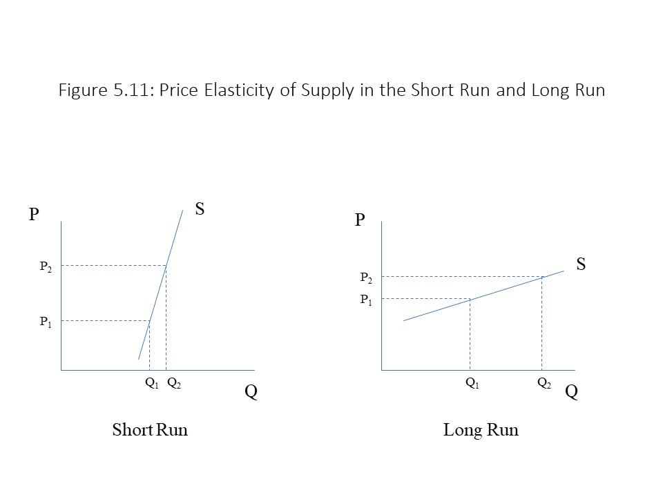 The
Cross-Price Elasticity of Demand
The
Cross-Price Elasticity of Demand