Describe short run production technology in the neoclassical tradition
Define the law of diminishing marginal returns to a single input
Explain how short run production technology generates short run production cost
Analyze different kinds of long run production technologies in the neoclassical tradition
Derive long run production cost from long run production technology
Demonstrate the relationship between short run and long run production cost
Investigate Schumpeterian and Marxian theories of production technology and cost
Short Run Production Technology in the Neoclassical Tradition
In the neoclassical tradition, production technology is defined very broadly to include all of the accumulated knowledge and technical skills that are used in the production of goods and services. As we will see, the unidirectional logic that is so central to neoclassical thinking applies in this case in that technology is used to determine the cost structure that firms face.
We begin with a distinction between two periods. The short run is a period in which at least one factor of production is fixed. If a pizzeria uses only capital (K) and labor (L), for example, we might expect labor to be a variable input whereas capital is its fixed input. That is, it may be possible for the firm to hire anywhere from 0 to a very large (unspecified) number of workers. At the same time, the restaurant itself, which includes its dining area, kitchen, and other facilities, is fixed in size. If the firm is not able to build a new restaurant or to add on to the existing restaurant, the firm is operating in the short run. If it takes 6 months to construct a new restaurant, then the short run in this specific industry is 6 months. The long run then refers to a period during which all factors of production are variable. In this example, the long run refers to a period that is longer than 6 months because both capital and labor are variable.
It is worth noting that the specific periods corresponding to the short run and the long run vary by industry. It may take two years to construct a new production plant in one industry and only six months to construct a new factory in a second industry. The amount of time simply depends on how long it takes for all inputs to become variable. It should also be emphasized that production technology remains fixed in both the short run and the long run. The knowledge and skills related to production do not change in this analysis, which is a key entry point of neoclassical theory. Also, consistent with the neoclassical approach is the assumption of a fixed capital endowment in the short run, which is another key entry point.
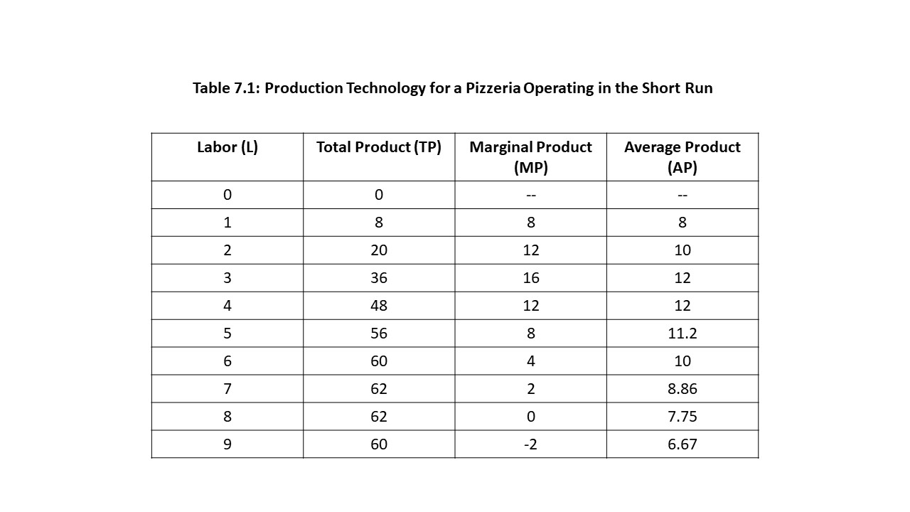
We will now continue with the example of a pizzeria in the short run. To represent the firm’s short run production technology, we will introduce a few key short run product concepts. The first concept is total product (TP). The total product refers to the total physical output produced during a given period, in this case a specific number of pizzas. In earlier chapters, we referred to total output as Q, which has the same meaning. Therefore, we can write the following:
An additional product concept that is critical for representing production technology in neoclassical theory is the concept of marginal product (MP). When an additional worker is hired, that additional worker increases total pizza production by a specific amount. This amount is the marginal product of that worker. For example, if the third worker increases total pizza production from 11 to 14 pizzas, then the marginal product of the third worker is 3 pizzas. Formally, we write the marginal product in the following way:
Finally, the concept of average product (AP) is important as well. In this example, the average product of labor refers to the average number of pizzas produced per worker. For example, if the total product is 30 pizzas and 10 workers are employed, then the average product is 3 pizzas per worker. It is important to understand the difference between average product and marginal product. Whereas marginal product only considers the addition to the total product of the last worker hired, average product spreads out the entire product evenly over the number of employed workers. The average product may be written as:
Table 7.1 provides an example with some hypothetical data for our pizzeria operating in the short run. Let’s say the period we are considering is one business day.
Using the information in the table, the MP when 3 workers are employed is calculated in the following way:
Similarly, the AP of the third worker is calculated as follows:
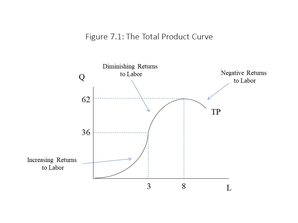
We are now able to consider the patterns that emerge from these calculations. The MP appears to rise until it reaches its peak at L = 3 workers. Next it declines, eventually reaching 0, and then becomes negative. The range over which MP rises is called the range of increasing returns to labor. The question arises as to why MP rises as more workers are hired at these low employment levels. The answer is specialization and the division of labor. Just think about all of the tasks that are involved in the pizza business. If a single worker is hired, then that worker needs to make the dough, roll the dough, toss the dough, make the sauce, spread the sauce, add the toppings, bake the pizza, cut the pizza into slices, take customer orders, serve the pizza to customers, bus the tables, wash the dishes, operate the register, clean the kitchen, clean the dining area, and clean the restrooms! The worker needs to accomplish other tasks as well, including ordering more ingredients, maintaining financial records, and paying taxes. Clearly, if a second worker is hired, then the tasks can be divided up, allowing for a greater degree of specialization. These gains from specialization imply that the second worker increases the TP by 12 pizzas, which is more than the increase that resulted from the hiring of the first worker. When three workers are hired, the tasks can be further divided so that one worker can work in the kitchen, a second worker can handle customer service in the dining area, and a third worker can work the cash register and maintain the books. As a result, the MP continues to rise. The reader should be aware that the additional workers hired are not more skilled or more hardworking. In fact, we are assuming the opposite. That is, each worker is equally skilled and hardworking. These gains in MP are solely the result of the benefits of specialization and the division of labor. The AP rises as well for this same reason.
Once we move beyond the point where three workers are hired, we begin to see a decline in the MP of labor. The range over which MP falls is called the range of diminishing returns to labor. Why does this decline in MP occur? Imagine that the kitchen is very small at our restaurant and the fourth worker is asked to work in the kitchen with the cook already present there. The worker contributes to production and so TP rises. At the same time, the presence of the additional worker in the kitchen makes it somewhat more difficult for the original cook to work efficiently. The two cooks keep running into one another. At times, they bump elbows as one rolls the dough and the other spreads the sauce. Even though the fourth worker adds to production, TP only rises by 12 pizzas rather than 16 pizzas as a result of this “bumping elbows problem.” The more formal phrase that is used to refer to this phenomenon is the law of diminishing returns to labor. It should be noted that AP falls for the same reason.
The law of diminishing returns may be expressed in two different ways. It may be expressed as:
a decline in the marginal product of labor as employment increases
an increase in the total product of labor at a diminishing rate
The reader should refer to Table 7.1 to observe these two patterns. It should be noted that this problem of bumping elbows eventually becomes so serious that the TP begins to fall. In other words, the MP becomes negative as additional workers reduce the total production of pizzas. The range of negative MP is referred to as the range of negative returns to labor. The underlying reason for this pattern of diminishing returns and then negative returns to labor is that the capital input (i.e., the size of the restaurant, and the kitchen, specifically) is fixed in the short run. The same pattern would eventually result if we were to add additional workers in the dining area and in the finance area. Due to the importance of the fixed capital input in generating this result, the law of diminishing returns is a specifically short run phenomenon.
It really should be emphasized how extraordinary the claim is that neoclassical economists are making when they assert that the law of diminishing returns holds for production technologies in the short run. They are claiming that every single short run production process exhibits this same pattern. It does not matter whether we are discussing the production of commercial aircraft, high-tech computers, cheese pizzas, automobiles, or haircuts. All these production processes have this basic feature of their production technologies in common. It is a fundamental aspect of our economic existence.
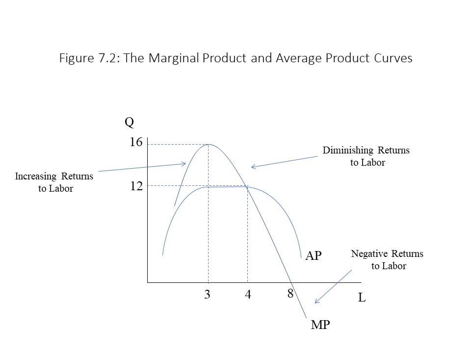
It is also possible to represent these patterns graphically. The TP curve that corresponds to the data in Table 7.1 is represented in Figure 7.1. The MP and AP curves corresponding to these data are represented in Figure 7.2.
It is important to notice that MP and AP intersect in Figure 7.2 at L = 4 when both the AP and the MP are equal to 12 pizzas per worker. It turns out that MP always intersects AP at the peak of AP. Why? It helps to consider a non-economic example first. Suppose that the total weight of everyone in a classroom of 30 people is 4,200 lbs. The average weight of a person in the room is then equal to 140 lbs. (= 4,200 lbs. / 30 people). Next let’s consider what would happen if we bring in a marginal person (person A) from outside the room. Person A is a football player who weighs 300 lbs. Notice that the total weight in the room is now 4,500 lbs. and the number of people in the room is 31 people. In that case, the new average weight will be approximately 145 lbs. (= 4,500 lbs. / 31 people). Because the marginal weight exceeded the average weight, the average weight rose. It follows that if the marginal contribution exceeds the average, the average will rise. In the case of MP and AP, if the MP exceeds the AP, the AP will rise.
If instead we had brought in a marginal person (person B) with a weight of 100 lbs., then the average weight of a person in the room would be approximately equal to 139 lbs. (= 4,300 lbs. / 31 people). Because the marginal weight is below the average weight in this example, the average weight falls. It follows that if the marginal contribution is below the average, the average will fall. In the case of MP and AP, if the MP is below the AP, the AP will fall.
In Figure 7.2, the reader can see that at low employment levels, the MP exceeds the AP causing the AP to rise. At higher employment levels, the MP falls below the AP causing the AP to fall. It follows that the MP must intersect the AP at the peak of the AP curve. To the left of the peak, the higher MP pulls the AP up and to the right of the peak, the lower MP pulls the AP down.
Short Run Production Cost in the Neoclassical Tradition
Our next task is to explain the cost structure that firms face in the short run. We will differentiate between two types of short run cost. First, total variable cost (TVC) refers to the total monetary cost of the variable input, which in this case is labor. If we assume a constant wage rate (w), measured in terms of dollars per worker, then TVC may be calculated as follows:
Because L can be measured in terms of the number of workers employed during this period, TVC is measured in dollars of labor cost incurred during this period. TVC can change in the short run because L is a variable input.
The other major type of cost is total fixed cost (TFC). TFC refers to the total monetary cost of the fixed input, which in this case is capital. If we assume a constant price of capital (PK), measured in terms of dollars per unit of capital, then TFC may be calculated as follows:
Because K is measured in terms of the number of units of capital employed during this period, TFC is measured in dollars of capital cost incurred during this period. With both K and PK fixed, the TFC is also fixed in the short run.
The firm’s total cost (TC) is simply the sum of TVC and TFC. It can be expressed as:
TC is measured in terms of dollars of cost incurred during this period.
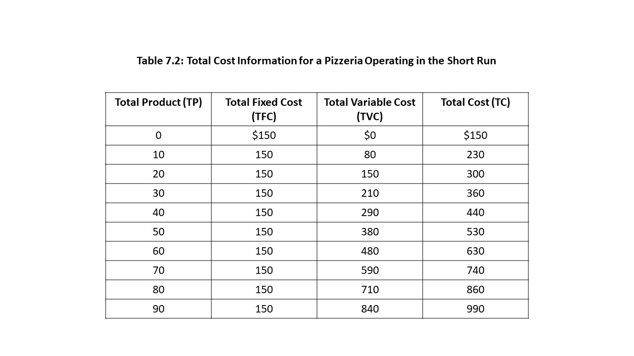
For example, we can select some hypothetical cost data for a pizzeria operating in the short run as shown in Table 7.2.[1]
If the numbers in Table 7.2 correspond to one business day, then the capital cost or TFC (i.e., the rent for the building) is fixed for all levels of output at $150 per day. The labor cost or TVC, on the other hand, rises with output because increased employment of the variable input is what makes possible the rise in output. Finally, total cost rises because the TVC is rising even though the TFC remains fixed. It should also be noted that TVC is $0 when 0 units of output are produced because no workers are hired, but TFC is still $150 because the rent must be paid regardless of whether pizzas are produced.
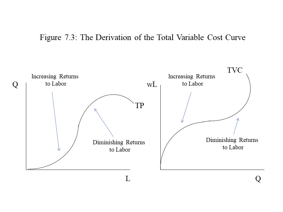
It is possible to say more about this pattern of short run production cost. In fact, we can use the short run production technology concepts already developed to derive a specific pattern of short run production cost. It is easiest to understand this derivation by considering the similarities between the TP curve and the TVC curve as shown in Figure 7.3.
First consider the axes in each of the graphs in Figure 7.3. The axes are essentially reversed in the two graphs. The only other difference is the multiplication of L by the w in the TVC graph. If w is $1 per worker, then this difference disappears. Even if the wage is some other value, the only result will be a stretching of the graph, but its basic shape will remain unchanged. Now consider the shapes themselves. The reader might imagine lifting the TP curve off the graph and twisting it around until it can be placed directly on top of the TVC curve. What this exercise implies is that the TVC curve possesses its shape for precisely the same reason that the TP curve possesses its shape. That is, at low output levels, TVC rises slowly due to the specialization and division of labor. At higher output levels, TVC rises more quickly due to diminishing returns to labor as it becomes necessary to hire more and more labor to increase production by given amounts.Figure 7.4.
Because the TFC is fixed at $150 for all levels of output, the TFC curve is simply a horizontal line. The TC curve, however, has the same shape as the TVC curve because TC only changes due to changes in TVC (since TFC is fixed). In addition, the TC curve is shifted upwards by the amount of the TFC. As a result, the distance between the TVC and TC curves is always equal to the TFC. Because the TFC is reflected in the distance between these two curves, it is not necessary to include the TFC curve when we wish to represent the three total cost measures on a single graph. For that reason, the TFC curve has been included here as a dotted line. Also, because all three concepts are measured in dollars, the “$” symbol has been placed on the vertical axis.
Next, we need to introduce several unit cost concepts. Often managers of firms think in terms of production cost per unit of output produced, particularly when they are considering whether to increase or decrease production by a small quantity. We will define four key unit cost concepts, and then we will consider the pattern these unit cost measures exhibit as output changes in the short run.
The first unit cost concept that we will define is average variable cost (AVC). The AVC is the variable cost per unit of output produced. If labor is the variable input, then the AVC is per unit labor cost. If total wages amount to $1000 and 100 units of output are produced, then the AVC is $10 per unit (= $1000/100 units). It is defined in the following way:
Another unit cost concept that we will define is average fixed cost (AFC). The AFC is the fixed cost per unit of output produced. If capital is the fixed input, then the AFC is the per unit capital cost. If total capital cost amounts to $4500 and 100 units of output are produced, then the AFC is $45 per unit (= $4500/100 units). It is defined in the following way:
A third unit cost concept that we will define is average total cost (ATC). The ATC is the total cost per unit of output produced. It is simply the sum of the AVC and the AFC. If the AVC is $10 per unit and the AFC is $45 per unit, then the ATC is $55 per unit (= 10+45). Alternatively, if total cost is $5500 and total output is 100 units, then ATC is $55 per unit (= $5500/100 units). It is defined as follows:
The final unit cost concept that we will define is marginal cost (MC). The MC is the additional total cost per additional unit of output produced. For example, if total cost rises by $200 and total output rises by 50 units, then MC is $4 per unit. Furthermore, because total cost can only rise due to a rise in variable cost (since TFC is fixed), the MC can also be defined as the additional variable cost per additional unit of output produced. It is thus defined as follows:
Using the total cost information presented in Table 7.2, we can now calculate all these additional unit cost measures for our pizzeria operating in the short run. Table 7.3 combines the total cost information from Table 7.2 with the corresponding unit cost calculations.
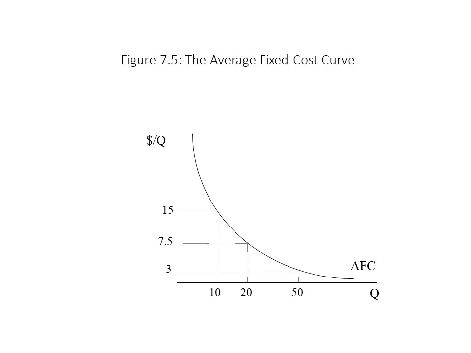
Clear patterns emerge for each of the unit cost concepts. The AFC, for example, declines continuously as total product rises. This reduction in AFC occurs because the fixed cost is spread over a larger and larger quantity of output. Businesspeople refer to this phenomenon of a falling AFC as “spreading one’s overhead.” Figure 7.5 shows a graph of the AFC curve.
As Figure 7.5 indicates, the AFC curve possesses horizontal and vertical asymptotes. That is, at very low output levels, the AFC soars because the denominator approaches zero while the numerator remains fixed (equal to TFC). As output rises, on the other hand, AFC declines due to the spreading of overhead. That is, output becomes increasingly large while the numerator remains fixed. The curve will never cross the horizontal axis though because some fixed cost will always exist no matter how thinly it is spread across the existing output. It should also be noted that $/Q has been placed on the vertical axis because the unit cost concepts are measured in dollars per unit of output.
In addition, Table 7.3 shows that the AVC, ATC, and MC measures all decrease at low output levels and then rise at higher output levels. Because they are derived from the total cost measures, the reductions in AVC and MC can be attributed to specialization and division of labor. The ATC falls at low output levels for two reasons. As the sum of AVC and AFC, it falls due to specialization and division of labor (falling AVC) and due to the spreading of overhead (falling AFC). All three measures begin to rise at higher output levels due to diminishing returns to labor.
As Figure 7.6 shows, the AVC, ATC, and MC curves are all U-shaped.
Furthermore, because the ATC is equal to the sum of AFC and AVC, it follows that AFC = ATC – AVC. Therefore, the difference between the ATC and AVC curves will always equal the AFC. As a result, we do not need to include the AFC curve when we wish to graphically represent the four unit-cost measures. For that reason, the AFC curve has been omitted in Figure 7.6. It should also be noticed that the AVC and ATC curves grow closer together as Q rises. The reason is that AFC is declining due to the spreading of overhead.
An additional point that must be made is that MC intersects AVC and ATC at the minimum points on the AVC and ATC curves. The reason is the same as that used to explain why MP intersects AP at the maximum AP. That is, when MC is below the AVC, the AVC falls. When the MC is above the AVC, the AVC rises. Therefore, the MC intersects the AVC at the minimum AVC. The same argument can be used to explain why MC intersects ATC at the minimum ATC. In terms of Table 7.3, we can see that MC changes from being below AVC to being greater than AVC between 30 and 40 units of output. The intersection of the two curves, therefore, occurs within that range. Similarly, MC changes from being below ATC to being greater than ATC between 60 and 70 units of output. The intersection of the MC and ATC curves must occur within that range as well.
Finally, the relationship between the product curves and cost curves should be emphasized once more. Because production technology determines production cost in neoclassical theory, we should be able to identify some connection between the product concepts and the unit cost concepts. It turns out that the MP and AP curves are the mirror image of the MC and AVC curves, respectively. If we look at the definitions, this implication leaps out at us.
Clearly, if ∆Q/∆L rises, then ∆L/∆Q falls. That is, if MP rises, then MC falls. The opposite also holds that if MP falls, then MC rises. We can make the same argument about the relationship between AP and AVC. That is:
It should be clear that if Q/L rises, then L/Q falls. Hence, a rise in AP coincides with a fall in AVC. The opposite also holds that if AP falls, then AVC rises. Figure 7.7 shows these curves side-by-side to emphasize the relationships between them.
Finally, we have been assuming the ceteris paribus condition throughout this analysis. That is, we have assumed that the wage rate, the price of capital, the quantity of capital, and the production technology have remained fixed. We should briefly consider what will happen to the unit cost curves if any of these factors changes. For example, a rise in wages will cause the AVC, ATC, and MC curves to shift upwards. The reason is that wages determine TVC, which influences the position of each of these curves. If wages rise, the firm faces higher unit costs. Second, a rise in the price of capital or in the quantity of capital employed will cause an upward shift of the ATC curve but will leave the AVC and MC curves unchanged. The reason is that these factors only affect the TFC, which influences the AFC but not the AVC or MC. Hence, the gap between the ATC and AVC curves will rise as AFC grows but otherwise nothing will change. Finally, a technological improvement will cause a reduction in the AVC and MC (and thus the ATC). Therefore, a downward shift of the AVC, MC, and ATC curves will occur. It is left to the reader to consider the consequences of a reduction in wages, the price of capital, or the quantity of capital employed. A loss of technological knowledge is also theoretically possible and should be considered.
A Short Run Technology and Cost Example Using Microsoft Excel
It is helpful to use a spreadsheet software program such as Microsoft Excel when analyzing the short run production technology and cost structure facing a firm. The reason is that it allows one to avoid performing all the calculations by hand, and so it saves the analyst a great deal of work. Let’s consider a simple example in which an analyst only has a small amount of information about a firm. Suppose the analyst only knows that the wage is $5 per hour and the price of capital (PK) is $2 per unit. That is, w = 5 and PK = 2. Suppose that the only other information the analyst possesses relates to total product and the capital stock as shown in Table 7.4.
In MS Excel, the columns are labeled with capital letters and the rows are numbered. The reader may be surprised to learn that the entire table can be completed with only the information that has been provided. To complete the entire table by hand would require 199 separate calculations! Fortunately, MS Excel allows us to use the definitions of each measure and then use cell references to complete the entire table in a small fraction of the time it would take to complete the table by hand.
Because the capital stock is fixed in the short run at all output levels, we can simply copy and paste that quantity of capital to every cell in column B. To carry out this operation quickly, it is only necessary to place the cursor over the lower right corner of the cell B2 until the cursor turns into a little black cross (+). The analyst may then drag the cursor all the way down the column until it is complete.
The other columns are a little more difficult to complete because it is necessary to insert a formula to ensure an accurate calculation. Whenever entering a formula in MS Excel, it is necessary to first include an “=” sign. For example, because the definition of AP is TP/L, the AP is calculated as =C2/A2 for L = 0. As with the capital stock, this formula can be dragged down to complete the rest of the cells in the column. The rest of the columns are completed in a similar fashion. It should be noted that the “*” symbol, which is used in the calculation of TVC and TFC, is used for the multiplication of terms in Excel.
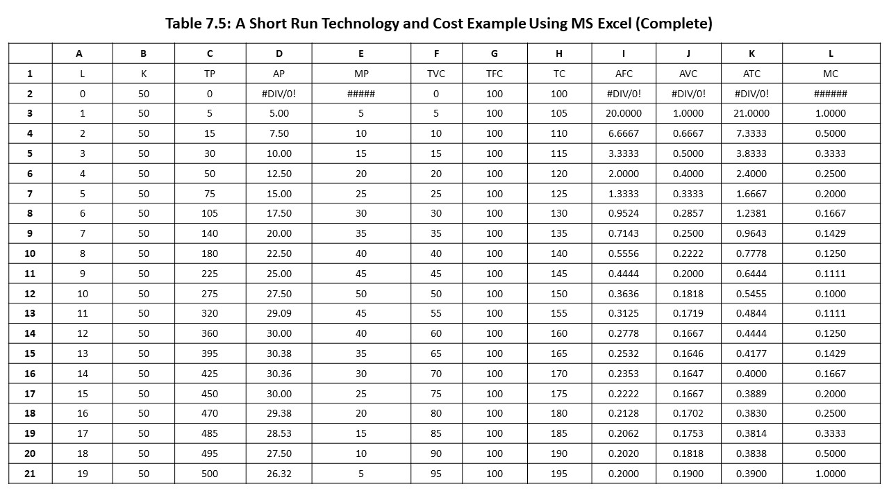
Table 7.5 shows the complete table after all calculations have been performed.
A few points worth noticing include the fact that diminishing returns to labor first appear at L = 11 when MP shows a decline for the first time. Additionally, it is also at this employment level that MC begins to rise for the first time, which demonstrates the notion that the MP and MC are mirror images of one another. Finally, it is possible to locate the points of intersection of MC with AVC and ATC. MC intersects AVC between employment levels 13 and 14, whereas MC intersects ATC between employment levels 17 and 18. The reader might notice that MP intersects AP between employment levels 13 and 14, a fact which also reinforces the point that the MP and AP curves are mirror images of the MC and AVC curves.
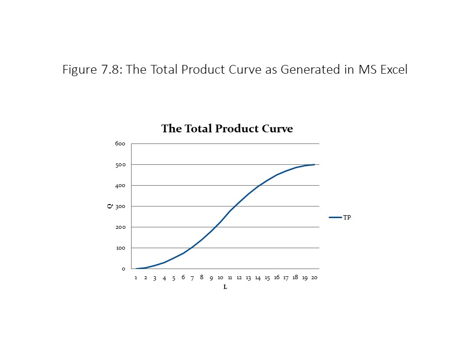
It is also possible to generate graphs in Excel of the product and cost curves. To illustrate how these graphs may be created, we will create a graph of the TP curve and a separate graph containing the AP and MP curves. To create a graph, the analyst should select the following:
On the Insert Tab, choose “Line.”
From the options available, choose “Line” again.
A chart box should appear. Right click it and choose “Select Data.”
Next click “Add” and in the new box type “TP” for Series Name.
Where it says, “Series Values,” click the symbol to the right and then drag in the data for TP from the Excel table beginning with L = 0. Then click OK and click OK once more.
To add horizontal and vertical axis labels, you can use the Design and Layout Tabs.
Figure 7.8 shows the TP curve as generated in MS Excel.
The same procedure may be used to create the graph of the AP and MP curves. The only difference is that you need to return to step 4 to “Add” the second curve after the first has been created. Also, because the values are undefined for L = 0, it is best to omit these calculations when dragging in the data for these two curves. Figure 7.9 shows the AP and MP curves as generated in Excel.
Long Run Production Technology in the Neoclassical Tradition
We now turn to production technology in the long run when all inputs are variable. In the case of the pizzeria, it is now technically possible for the firm to construct additional restaurants in addition to hiring additional workers. We will discuss three types of long run production technologies before we explain how these long run technologies determine long run production costs.
The first type of long run production technology is a technology that exhibits constant returns to scale (CRS). A CRS technology exists when a fixed percentage change in all inputs leads to the same percentage change in total output. For example, suppose that the amounts of capital and labor double (100% increases in each). In that case, the amount of output produced also exactly doubles, assuming a CRS technology. Using the pizzeria example, if 3 workers in one restaurant produce 10 pizzas in an hour, then 6 workers in two restaurants will produce 20 pizzas in an hour, assuming a CRS technology. The assumption of a CRS technology should seem reasonable enough. A firm should be able to perfectly duplicate its smaller scale operation when it doubles its inputs and so output should exactly double.
A second type of long run production technology is a technology that exhibits increasing returns to scale (IRS). An IRS technology exists when a fixed percentage change in all inputs leads to a greater percentage change in total output. For example, suppose that the amounts of capital and labor double (100% increases in each). In that case, the amount of output produced more than doubles, assuming an IRS technology. It may seem strange, given what was previously explained about the likely consequences of duplication, that output could more than double. It would be relatively easy to explain this possibility with an impure example. That is, we might argue that the quantities of labor and capital have exactly doubled but the qualities of the newly acquired capital and labor are superior to what was previously used, causing output to more than double.
It is possible, however, to provide a pure example of an IRS technology or one in which a doubling of the inputs leads to a greater than doubling of output even when the additional inputs are of the same quality as that which was previously used. Such cases arise when the production processes have certain geometric characteristics that make IRS technologies possible.[2] For example, consider an oil pipeline that transports oil over a long distance. To keep the example simple, we will focus on the opening at one end of the pipeline, which is assumed to form a perfect circle. The circumference of the circle (i.e., the distance around it) is directly related to the amount of material that is used to construct the pipeline. That is, a larger circumference implies a larger amount of material that is required to produce the pipeline. The circumference (C) is given by the following formula where r is the radius of the circle:
The area of the circle, by contrast, is directly related to the amount of oil that can pass through the pipeline. That is, a larger opening implies that a larger amount of oil can pass through the pipeline. The area of the circle is given by the following formula:
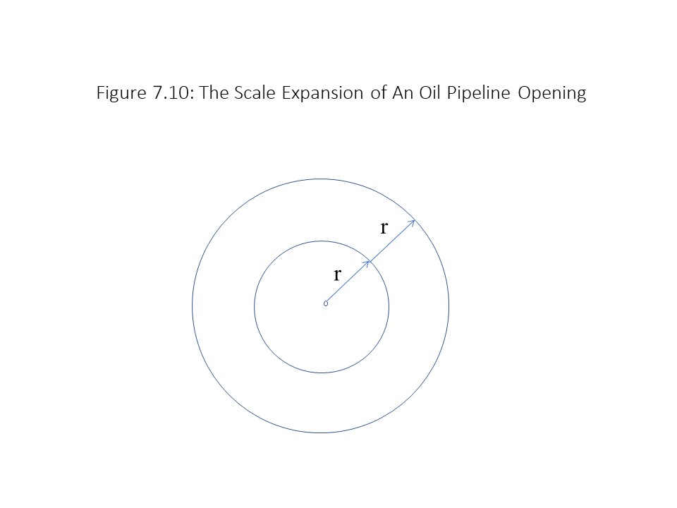
Now consider what happens when we double the amount of material used in the construction of the pipeline. This doubling of the amount of material makes possible a doubling of the circumference of the circle. In Figure 7.10, the inner circle represents the original pipeline opening and the outer circle represents the new pipeline opening that uses twice as much material.
According to the figure, the doubling of the circumference doubles the radius of the circle. As a result, we can calculate the circumference of the larger opening (C’) as:
In other words, the doubling of the radius has doubled the circumference, which indicates that the amount of material inputs has doubled. What effect does this doubling of the radius have on the area of the new opening? We can calculate the area of the larger opening (A’) as follows:
In other words, the doubling of the radius leads to a quadrupling of the area of the opening. That is, the material inputs in the production of the pipeline have doubled and yet the output that passes through the pipeline has more than doubled. It appears we have a pure example of an increasing returns to scale (IRS) technology.
The third and final type of long run production technology is a technology that exhibits decreasing returns to scale (DRS). A DRS technology exists when a fixed percentage change in all inputs leads to a smaller percentage change in total output. For example, suppose that the amounts of capital and labor double (100% increases in each). In that case, the amount of output produced lessthan doubles, assuming a DRS technology. It is difficult to provide pure examples of DRS technologies, although it is relatively easy to provide any number of impure examples. That is, we might argue that the quantities of labor and capital have exactly doubled but the qualities of the newly acquired capital and labor are inferior to what was previously used, causing output to less than double. More will be said about these issues when we discuss long run production cost.
Table 7.6 provides a summary of the three types of long run production technologies.
In each of the three cases (2A, 2B, and 2C), the quantities of capital and labor exactly double, but the output responds differently in each case. In the case of CRS, output exactly doubles. In the case of IRS, output triples. Finally, in the case of DRS, output only rises by 50%.
Long Run Production Cost in the Neoclassical Tradition
We are now able to draw some conclusions about long production cost based on our discussion of long run production technology. As in the short run, production technology determines the pattern of production cost that the firm faces. The most important long run cost concept that we will explore is long run average total cost (LRATC). As in the short run, average total cost in the long run is simply total cost per unit of output. The only difference is that LRATC may change due to a change in capital cost or due to a change in labor cost. It is defined as follows:
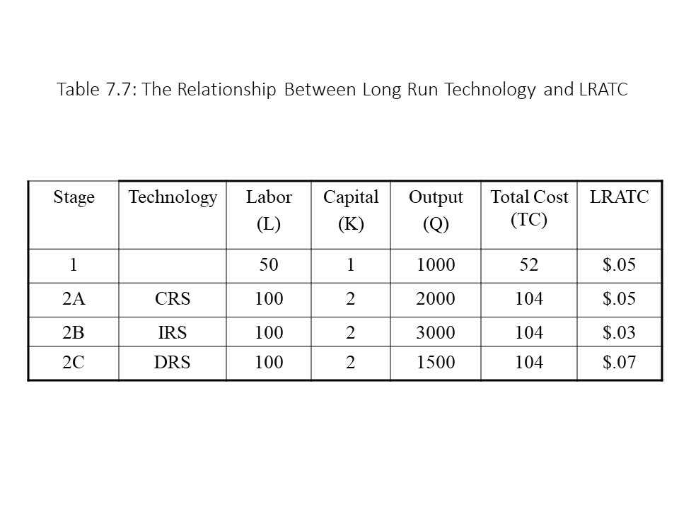
Let’s assume that the factor prices are constant in the long run such that w = 1 and PK = 2. We can now see clearly what the relationship is between the three types of long run production technology and LRATC. Table 7.7 shows the calculations for TC and LRATC for each of the three cases considered previously in Table 7.6.
What this example shows clearly is that total cost exactly doubles in all three scenarios because the inputs have exactly doubled. It is the changes in output that differ in all three scenarios, which causes the LRATC to be different in the three cases. Specifically, we see that an increase in the scale of production leaves LRATC unchanged at $0.05 per unit in the case of a CRS technology. Because TC and Q grow at the same rate, the ratio of the one to the other does not change. By contrast, an increase in the scale of production causes the LRATC to fall from $0.05 to $0.03 per unit in the case of an IRS technology. The reason is that TC grows more slowly than Q and so the ratio of TC to Q declines. Finally, an increase in the scale of production causes the LRATC to rise from $0.05 to $0.07 per unit in the case of a DRS technology. The reason is that TC grows more quickly than Q and so the ratio of TC to Q rises.
The calculations from this example can be summarized as follows:
Special phrases are used to describe changes in LRATC as the scale of production changes:
Economies of scale (EOS) refer to reductions in per unit cost as output rises.
Diseconomies of scale (DOS) refer to increases in per unit cost as output rises.
When per unit cost does not change with an expansion in the scale of production, the firm is said to experience neither EOS nor DOS.
Next, we should consider which of these cost patterns is most likely for an individual firm. Neoclassical economists argue that firms typically pass through all three phases as the scale of production grows. Specifically, firms experience scale economies at relatively low output levels, then they experience neither EOS nor DOS, and finally, they experience diseconomies of scale at relatively high output levels. Graphically, this pattern gives rise to a U-shaped LRATC curve like the one shown in Figure 7.11.
Why do neoclassical economists assert that this pattern of unit cost is a typical one facing firms? They give several reasons for expecting scale economies at relatively low output levels.[3] The first is labor and managerial specialization. Unlike in the short run, these types of specialization require that all inputs be variable. For example, imagine a firm that carries out both production and distribution activities in a single facility. As it expands in the long run and increases its capital stock, it might be able to carry out production in one facility and distribution in another facility. The gains from specialization may be considerable. As a result, TC grows more slowly than Q and LRATC falls.
Another reason for scale economies at relatively low output levels may be large startup costs. For example, in the automobile industry a huge outlay of financial capital is required to even begin operations. As more automobiles are produced, this initial outlay can be spread over a larger number of units and LRATC falls. Large startup costs in the long run operate in a similar manner to TFC in the short run.
As firms become larger, they also frequently enjoy efficiencies that stem from expanded knowledge of the production process. That is, they simply become more efficient producers as the kinks in the production process are worked out. As a result, TC rises less quickly than Q and LRATC falls. Other factors that contribute to scale economies have more to do with input prices. For example, as firms expand they can take advantage of bulk discounts that suppliers offer. Another possibility is that they can borrow funds more cheaply in the stock and bond markets than smaller firms, which must rely on bank financing. As a result, output grows more quickly than cost and LRATC falls.
On the other end of the spectrum are scale diseconomies, which can arise for a variety of reasons. First, corporate bureaucracies may become excessively large as the scale of production expands. If highly paid top executives are hired to prepare a lot of paper reports, the result may be a considerable rise in TC without much expansion of Q. In that case, LRATC rises. Communication problems are another potential source of DOS in large organizations. If managers have a difficult time coordinating production due to the large size, then further expansion may raise TC more than Q.
The alienation that workers experience in the workplace in very large organizations may be another problem. Poor work performance may result when workers feel disconnected from one another and from their work. The sense of alienation may become so great that Q rises slowly even as TC increases with the purchase of additional inputs. The additional cost of hiring supervisors to monitor worker performance in these situations may also add to cost. Although Marxists tend to emphasize worker alienation to a much greater degree than neoclassical economists, neoclassical economists sometimes recognize that this factor contributes to DOS.[4]
Finally, input prices may also be involved in creating DOS. For example, as firms expand to very large sizes, they may begin to push up input prices due to their increased demand for inputs. Similarly, if their large sizes necessitate transporting goods to more distant markets, then TC may rise more quickly than output.[5]
The Relationship between Short Run and Long Run Average Total Cost
The LRATC curve is sometimes described as the lower envelope of all short run average total cost (SRATC) curves. To understand the reason, consider Figure 7.12.
Figure 7.12 shows a series of SRATC curves, each corresponding to a different production plant size. As production increases in the short run for a firm operating with plant size 1, unit cost declines due to labor specialization within the plant. Eventually, diminishing returns begin to set in as output expands due to the fixed amount of capital, and unit cost rises. In the long run, however, the firm has the option of building a larger production plant, which allows the firm to move to plant size 2. As a result, unit cost begins to decline again due to specialization within the larger plant. Eventually, however, diminishing returns result, and unit cost begins to rise. The firm can expand in the long run by building an even larger production plant, and the same process repeats itself. Due to this analysis, we can trace out the lower envelope of the SRATC curves to obtain the LRATC curve.
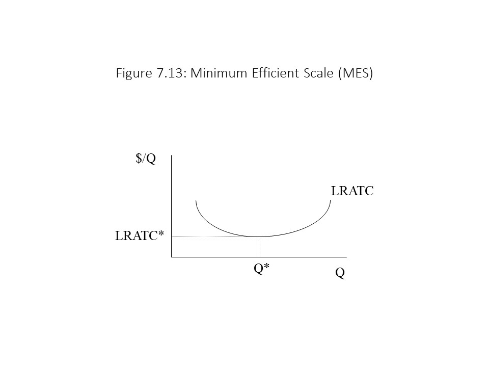
Minimum Efficient Scale
A final concept that deserves attention is what neoclassical economists call minimum efficient scale (MES). The MES refers to the lowest output level at which LRATC is minimized. Figure 7.13 shows the MES to be Q* because it is the lowest output level that minimizes LRATC.
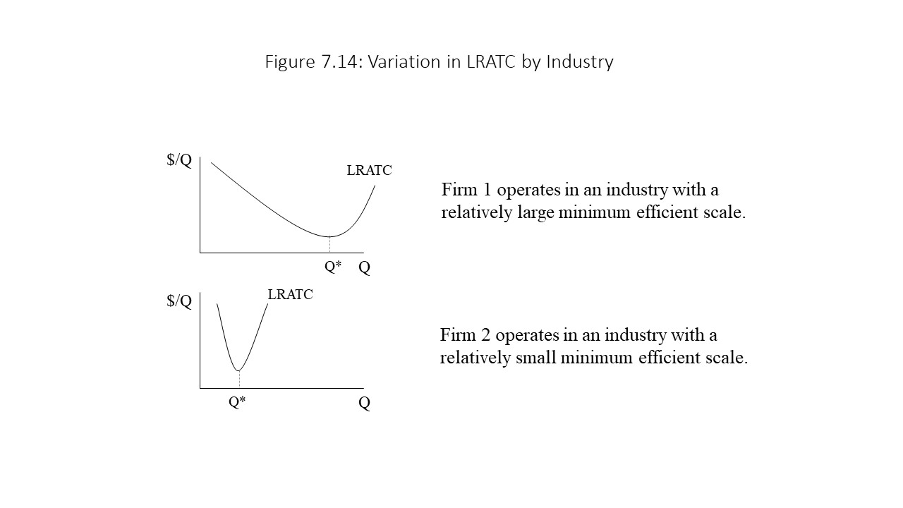
The MES varies by industry. For example, the MES has been estimated to be 10 million tons per year in the oil industry, 9 million tons per year in the steel industry, and at least 1 million barrels per year in the beer industry.[6] The MES in an industry may, therefore, be a large amount of output or a small amount of output. For example, Figure 7.14 contains examples of two LRATC curves. Each represents the LRATC of a firm in a different industry. Firm 1’s LRATC curve shows that the MES is very large due to large economies of scale in this industry. Only large firms in this industry will be able to minimize unit cost. Firm 2’s LRATC curve suggests a very small MES due to significant diseconomies of scale in this industry. Only small firms will be able to minimize unit cost in this industry.
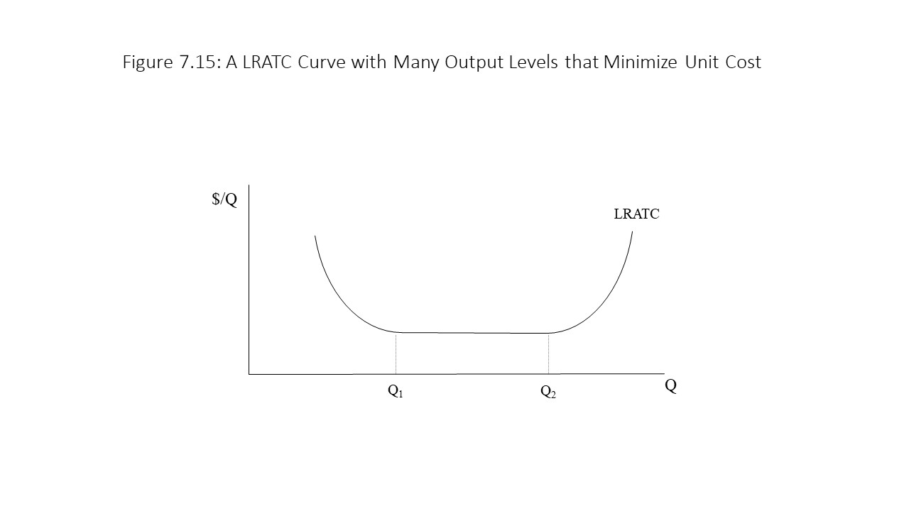
Furthermore, a firm may have multiple production levels that are consistent with minimum LRATC. For example, the firm’s LRATC curve shown in Figure 7.15 indicates that Q1 is the minimum efficient scale, but Q2 represents the maximum efficient scale.
That is, Q2 is the largest output level that still manages to keep unit cost at its minimum. In this industry, small firms, large firms, and medium-sized firms can operate at minimum unit cost.
The Schumpeterian Approach to Technological Change
The neoclassical theory of production technology and cost of production that we have been considering treats technology as completely static. Almost no emphasis is placed on technological change. Granted, neoclassical economists have more to say about technological change in macroeconomics, but in microeconomics it plays essentially no active role at all. For this reason, many heterodox economists challenge the neoclassical treatment of production technology.
One important example of an economist with a different approach to production technology is the famous economist Joseph Schumpeter, who is best known for his book, The Theory of Economic Development, first published in 1913. According to Schumpeter, technological change is the driving force in economies that creates economic growth, unstable and uneven as it is. Meghnad Desai provides a nice overview of Schumpeter’s theory:
Innovations often clustered together and made for an Industrial Revolution. But they came only periodically and discontinuously, in waves. One wave of innovations would break the mould of the old stationary economy. The pioneers would borrow money and launch their innovations. They would enjoy a temporary monopoly, and make immense profits (if, that is, they were successful, since there are also failures in this life). These innovations would launch the economy on a growth path with an upswing that might last twenty to twenty-five years. But imitators would soon come in and erode the entrepreneurs’ excess profits. Output would multiply, but prices would start falling and profits would go down. A downswing would set in until another wave of innovations hit the economy.[7]
According to Schumpeter, innovation would lead to long periods of growth and progress followed by periods of falling prices and sluggish growth until a new series of innovations revived the growth of capitalism. When innovation does occur, it generates growth in the innovating sectors but leads to “creative destruction” for the sectors made obsolete by the new technology. Clearly, Schumpeter’s theory shifts our focus to macroeconomics and away from microeconomics, but his theory also reveals just how static and unhelpful the microeconomic theory of production technology is when it comes to explaining technological progress.
A Marxian Approach to Technological Change
Much can be said regarding Marx’s thoughts about the role of technological change in capitalist economies and its ability to revolutionize the means of production. Indeed, Marx was a major influence on Schumpeter. When considering the specifically microeconomic aspects of production technology on which neoclassical economists focus, however, we will also find it helpful to contrast with those aspects the competing theory of production technology that is found in Marx’s work.
In chapter 3, it was explained that a commodity’s value is determined by the socially necessary abstract labor time (SNALT) required for its production. John Eatwell refers to Marx’s concept as one of “socially necessary technique.”[8] Some producers will devote more labor to production than is socially necessary. Other producers will devote less labor to production than is socially necessary. All producers, however, will receive a value in exchange that is based on the average degree of skill and intensity of labor prevailing in the industry at that point in time. Therefore, producers that use less labor than the social average will enjoy a surplus profit whereas producers that use more labor than the social average will experience a smaller than normal profit. Those producers that use an amount of labor that is exactly equal to the social average will enjoy a normal profit (determined by the amount of surplus value embodied in the commodity).
Because of these discrepancies, the producers will try their best to imitate the techniques of the most efficient producers. The surplus profits will be too tempting. If some of the producers succeed in their imitation of the other producers, then the SNALT embodied in the commodity will decline over time and its value will fall as well.
The value of the commodity is, of course, determined by the average producer. Over time, all producers manage to lower the SNALT that they must perform to produce the commodity as they try to imitate the lowest cost producer and as the lowest cost producer strives for even lower costs. The result is a steady decline in the value of the commodity. In this competitive environment, the surplus profits of the low-cost producer do not rise, even though she is innovating, because the value of the commodity is falling. Similarly, the lower-than-average profits of the high-cost producer persist, even though she is also innovating, because the value of the commodity is falling.
Consider an example that includes a high-cost producer, a low-cost producer, and an average producer. The product of the high-cost producer has an individual, private value of $25 whereas the product of the low-cost producer has an individual, private value of $15. The product of the average producer, however, has an individual, private value of $20. Because the value of the product of the average producer governs the market value, all three producers sell their commodities for $20 each. The low-cost producer thus receives a surplus profit of $5. The average producer does not receive any surplus profit but rather just a normal profit. Finally, the high-cost producer receives $5 less than a normal profit. Over time, technological innovation might cause all the individual, private values to decline by $5. The result will be a reduction in the market value without any change to the surplus profits of each producer. If the degree of technological innovation among the firms differs, however, then the surplus profits of each firm may change.
The world is experiencing a serious food crisis as close to 1 billion people experience severe hunger and roughly an additional billion people are not receiving enough key nutrients. The problem is expected to worsen in the coming decades as the human population continues to increase. With a fixed amount of land for cultivation, the problem of diminishing returns to land makes it difficult to increase food production sufficiently to keep up with global needs. In the past, the problem of diminishing returns to land has not become too serious because of technological advances in agriculture. The problem is that climate change is now threatening to interfere with productivity in agriculture, especially in poor nations. According to Siddharth Chatterjee, “it is estimated that climate change could reduce yields from rain-fed agriculture by 50 percent by 2020, jeopardizing the welfare of seven in ten people who depend on farming for a living.” Chatterjee explains that when crops are lost, families lose their ability to earn a living, which leaves children vulnerable to a variety of health problems, including malnutrition and malaria. As Chatterjee argues, technological change will become more important in the future to increase the resilience to climate-related shocks and raise productivity in Africa’s agricultural sector. Still, the problem of global hunger exists for reasons that go beyond diminishing returns to land, the slow pace of technological change, and climate change. The persistence of mass hunger even when large food surpluses exist in some countries is the result of uneven economic development and problems with the distribution of food to poorer regions.[10] If the global food distribution system responds to market demand rather than human need, we have every reason to expect a continuation of the global food crisis.
Summary of Key Points
In the short run, at least one input is fixed whereas in the long run, all inputs are variable.
The increasing marginal product of labor is due to specialization and division of labor whereas diminishing returns to labor is due to the inefficiencies resulting from using too much of a variable input with a fixed input.
When a marginal contribution exceeds the average, the average will rise. When a marginal contribution falls below the average, the average will fall.
Short run unit cost curves fall initially due to the specialization and division of labor, and they rise eventually due to diminishing returns to labor.
Constant, increasing, and decreasing returns to scale are three long run technologies that specify how output changes when all inputs change by a given percentage.
Economies and diseconomies of scale describe how unit cost changes as the scale of production changes.
Schumpeter asserts that technological innovations are the driving force behind economic development, but this development is highly cyclical.
In Marxian theory, competition and technological imitation in an industry will reduce the SNALT required for production and cause the value of a commodity to decline over time.
List of Key Terms
Production technology
Short run
Long run
Total product (TP)
Marginal product (MP)
Average product (AP)
Increasing returns to labor
Specialization and division of labor
Diminishing returns to labor
Law of diminishing returns
Negative returns to labor
Total variable cost (TVC)
Total fixed cost (TFC)
Total cost (TC)
Average variable cost (AVC)
Average fixed cost (AFC)
Average total cost (ATC)
Marginal cost (MC)
Constant returns to scale (CRS)
Increasing returns to scale (IRS)
Decreasing returns to scale (DRS)
Long run average total cost (LRATC)
Economies of scale (EOS)
Diseconomies of scale (DOS)
Short run average total cost (SRATC)
Minimum efficient scale (MES)
Maximum efficient scale
Problems for Review
1.Is it possible for the marginal product of labor to fall while the average product of labor rises? Explain the reason for your answer.
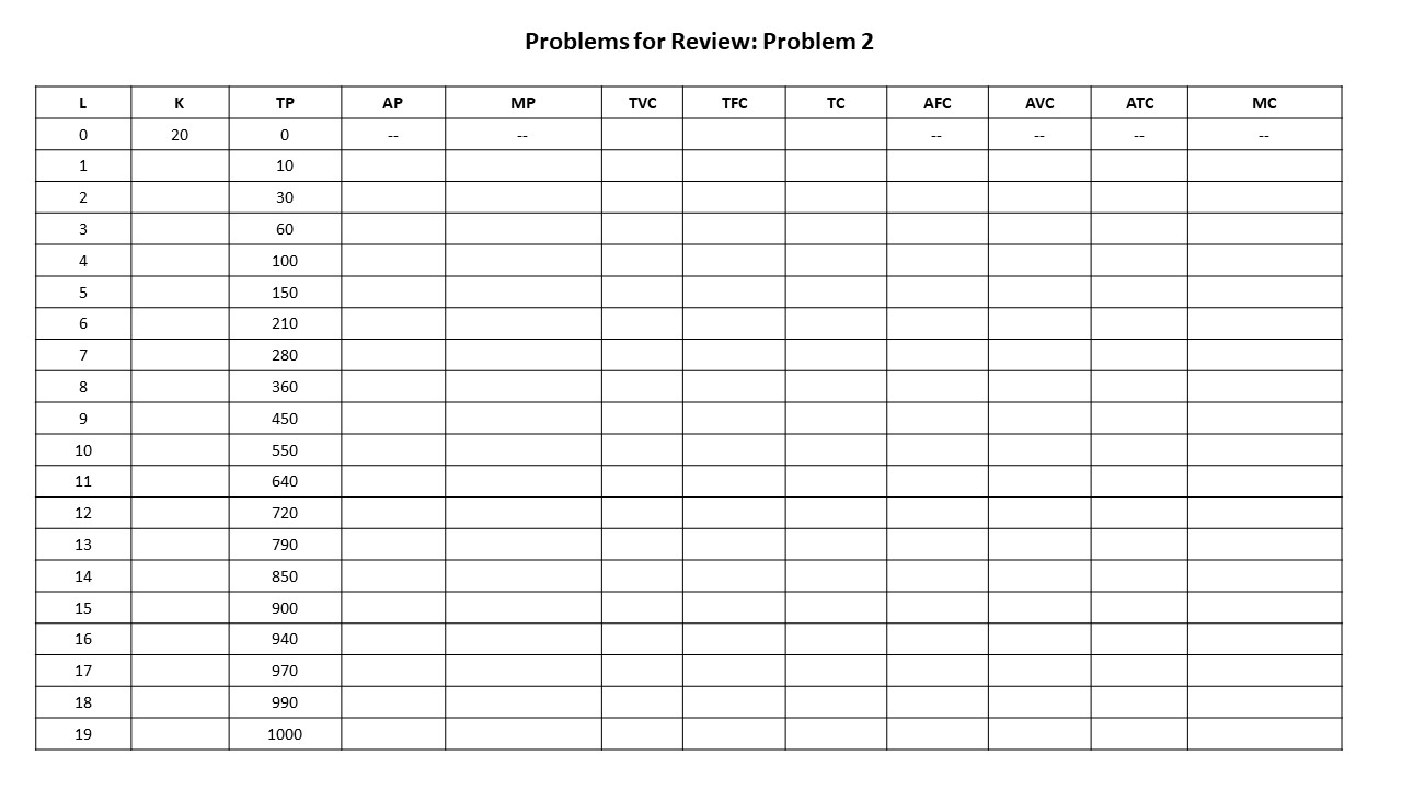
2. The table below represents the short run technology available to a firm. Assume that L is the variable factor of production and K is the fixed factor of production. The price of labor is $6 per unit and the price of capital is $4 per unit. Using a spreadsheet computer program (such as Microsoft Excel), complete the rest of the table.
3. Using the spreadsheet program you created to fill in the table in problem 2, create the two graphs described below in MS Excel. Remember to label all axes and curves.
The total product (TP) curve
The average product (AP) and marginal product (MP) curves (on one graph)
4. In the table from problem 2, what is the level of employment at which diminishing returns begin? What happens to the marginal product of labor and to marginal cost at this employment level?
5. Using the table from problem 2, fill in the blanks. Marginal cost equals minimum AVC between employment levels ____ and ____. Marginal cost equals minimum ATC between employment levels ____ and ____.
6. Suppose a firm hires only labor and capital and that the price of labor is $8 and the price of capital is $12. In the long run, the firm doubles its workforce from 8 to 16 units and doubles its capital from 12 to 24 units. Its output subsequently increases from 100 to 210 units.
What sort of technology is this firm using?
Calculate the firm’s long run average total cost before and after it changes its inputs.
These data are not intended to be compatible with the data in Table 7.1. ↵
See OpenStax College (2014), p. 170, for a similar application to the chemical industry. Examples of IRS technologies arising from these geometric properties are found in many neoclassical textbooks. ↵
These reasons are commonly cited in neoclassical economics textbooks. ↵
For example, see McConnell and Brue (2008), p. 393., and Lipsey and Courant, p. 179. ↵


 First consider the axes in each of the graphs in Figure 7.3. The axes are essentially reversed in the two graphs. The only other difference is the multiplication of L by the w in the TVC graph. If w is $1 per worker, then this difference disappears. Even if the wage is some other value, the only result will be a stretching of the graph, but its basic shape will remain unchanged. Now consider the shapes themselves. The reader might imagine lifting the TP curve off the graph and twisting it around until it can be placed directly on top of the TVC curve. What this exercise implies is that the TVC curve possesses its shape for precisely the same reason that the TP curve possesses its shape. That is, at low output levels, TVC rises slowly due to the specialization and division of labor. At higher output levels, TVC rises more quickly due to diminishing returns to labor as it becomes necessary to hire more and more labor to increase production by given amounts.
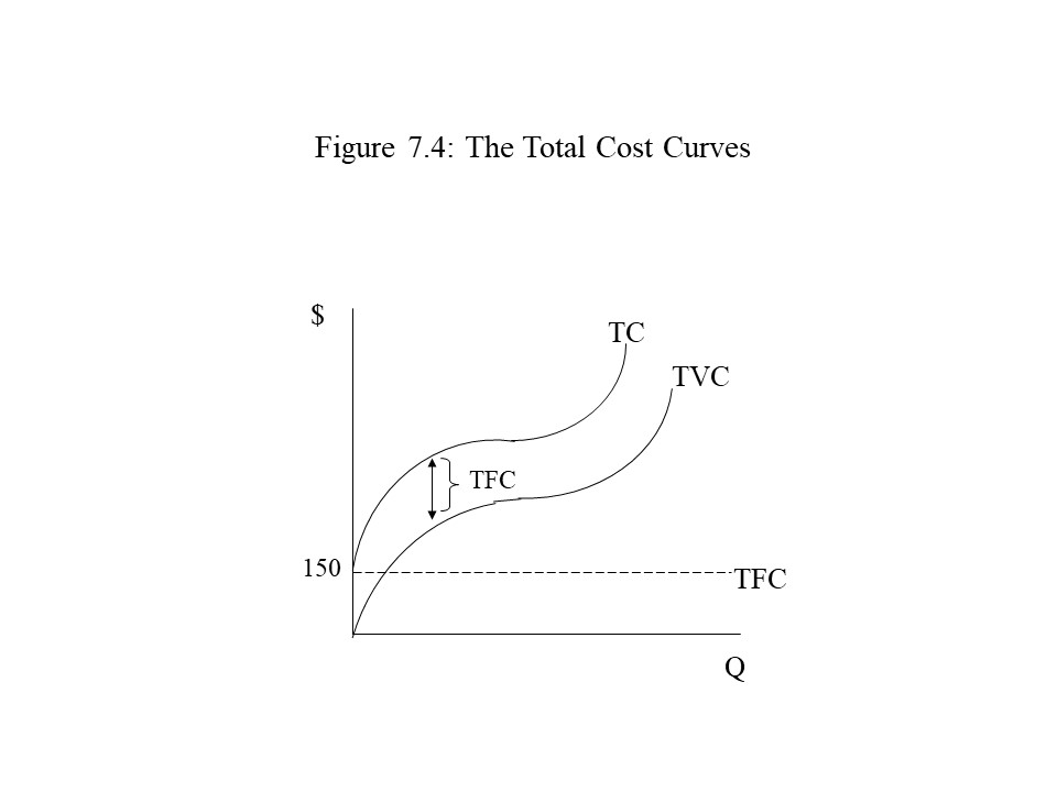 Because the TFC is fixed at $150 for all levels of output, the TFC curve is simply a horizontal line. The TC curve, however, has the same shape as the TVC curve because TC only changes due to changes in TVC (since TFC is fixed). In addition, the TC curve is shifted upwards by the amount of the TFC. As a result, the distance between the TVC and TC curves is always equal to the TFC. Because the TFC is reflected in the distance between these two curves, it is not necessary to include the TFC curve when we wish to represent the three total cost measures on a single graph. For that reason, the TFC curve has been included here as a dotted line. Also, because all three concepts are measured in dollars, the “$” symbol has been placed on the vertical axis.
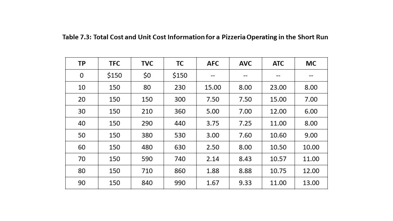
 As Figure 7.5 indicates, the AFC curve possesses horizontal and vertical asymptotes. That is, at very low output levels, the AFC soars because the denominator approaches zero while the numerator remains fixed (equal to TFC). As output rises, on the other hand, AFC declines due to the spreading of overhead. That is, output becomes increasingly large while the numerator remains fixed. The curve will never cross the horizontal axis though because some fixed cost will always exist no matter how thinly it is spread across the existing output. It should also be noted that $/Q has been placed on the vertical axis because the unit cost concepts are measured in dollars per unit of output.
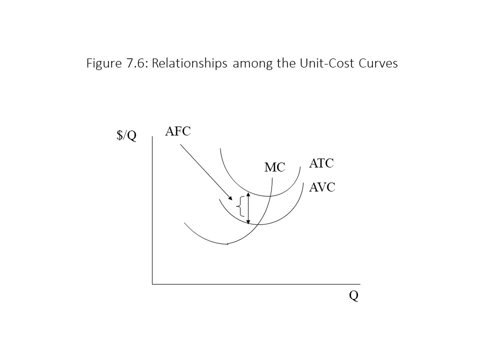 Furthermore, because the ATC is equal to the sum of AFC and AVC, it follows that AFC = ATC – AVC. Therefore, the difference between the ATC and AVC curves will always equal the AFC. As a result, we do not need to include the AFC curve when we wish to graphically represent the four unit-cost measures. For that reason, the AFC curve has been omitted in Figure 7.6. It should also be noticed that the AVC and ATC curves grow closer together as Q rises. The reason is that AFC is declining due to the spreading of overhead.
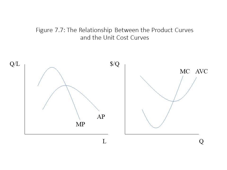 Finally, we have been assuming the ceteris paribus condition throughout this analysis. That is, we have assumed that the wage rate, the price of capital, the quantity of capital, and the production technology have remained fixed. We should briefly consider what will happen to the unit cost curves if any of these factors changes. For example, a rise in wages will cause the AVC, ATC, and MC curves to shift upwards. The reason is that wages determine TVC, which influences the position of each of these curves. If wages rise, the firm faces higher unit costs. Second, a rise in the price of capital or in the quantity of capital employed will cause an upward shift of the ATC curve but will leave the AVC and MC curves unchanged. The reason is that these factors only affect the TFC, which influences the AFC but not the AVC or MC. Hence, the gap between the ATC and AVC curves will rise as AFC grows but otherwise nothing will change. Finally, a technological improvement will cause a reduction in the AVC and MC (and thus the ATC). Therefore, a downward shift of the AVC, MC, and ATC curves will occur. It is left to the reader to consider the consequences of a reduction in wages, the price of capital, or the quantity of capital employed. A loss of technological knowledge is also theoretically possible and should be considered.
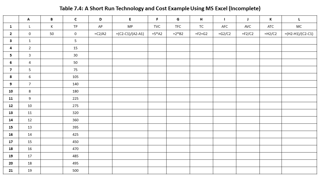
 The same procedure may be used to create the graph of the AP and MP curves. The only difference is that you need to return to step 4 to “Add” the second curve after the first has been created. Also, because the values are undefined for L = 0, it is best to omit these calculations when dragging in the data for these two curves. Figure 7.9 shows the AP and MP curves as generated in Excel.
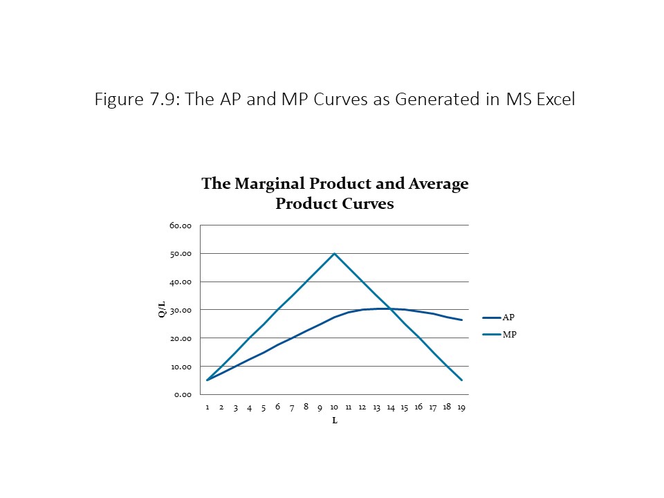
 According to the figure, the doubling of the circumference doubles the radius of the circle. As a result, we can calculate the circumference of the larger opening (C’) as:
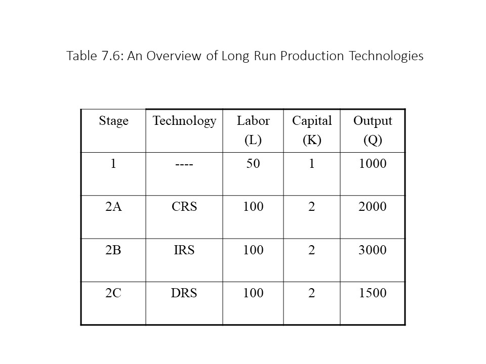
 What this example shows clearly is that total cost exactly doubles in all three scenarios because the inputs have exactly doubled. It is the changes in output that differ in all three scenarios, which causes the LRATC to be different in the three cases. Specifically, we see that an increase in the scale of production leaves LRATC unchanged at $0.05 per unit in the case of a CRS technology. Because TC and Q grow at the same rate, the ratio of the one to the other does not change. By contrast, an increase in the scale of production causes the LRATC to fall from $0.05 to $0.03 per unit in the case of an IRS technology. The reason is that TC grows more slowly than Q and so the ratio of TC to Q declines. Finally, an increase in the scale of production causes the LRATC to rise from $0.05 to $0.07 per unit in the case of a DRS technology. The reason is that TC grows more quickly than Q and so the ratio of TC to Q rises.
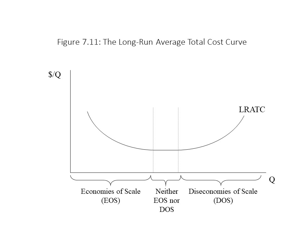
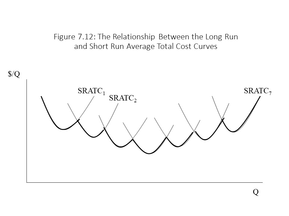 Figure 7.12 shows a series of SRATC curves, each corresponding to a different production plant size. As production increases in the short run for a firm operating with plant size 1, unit cost declines due to labor specialization within the plant. Eventually, diminishing returns begin to set in as output expands due to the fixed amount of capital, and unit cost rises. In the long run, however, the firm has the option of building a larger production plant, which allows the firm to move to plant size 2. As a result, unit cost begins to decline again due to specialization within the larger plant. Eventually, however, diminishing returns result, and unit cost begins to rise. The firm can expand in the long run by building an even larger production plant, and the same process repeats itself. Due to this analysis, we can trace out the lower envelope of the SRATC curves to obtain the LRATC curve.