Identify the defining characteristics of monopolies and barriers to the entry of competitors
Explain the nature of the demand facing a monopolist and its marginal revenue
Apply the rules of short run profit maximization for a monopolist to a variety of situations
Explore the implications of monopoly for efficiency and the long run
Analyze the special cases of natural monopoly and price discriminating monopoly
Investigate the Austrian and Randian critiques of neoclassical monopoly theory
Examine the Marxian theory of monopoly capital
Neoclassical Monopoly Theory: Defining Characteristics and Types of Entry Barriers
In the nineteenth century, competition in many American industries was quite fierce. As firms implemented new production technologies and new firms entered markets to capture a share of the profits, prices fell and the competitive struggle drove many firms out of business. In the iron and steel industry, for example, many iron and steel companies entered pricing pools in an effort to place limits on price competition. These agreements were not very stable, however, and by the late nineteenth century, a wave of mergers swept through American industry as firms strove for a way to stabilize their prices and profits. Out of this merger wave arose several giant corporations in a variety of different industries. These firms controlled such a large part of the total output of their industries that observers regarded them as monopolies. For example, the United States Steel Corporation (known simply as U.S. Steel) controlled most steel production in the United States after its formation in 1901. Other examples include International Harvester, which dominated the agricultural machinery market, and American Tobacco, which was dominant in the cigarette market. John D. Rockefeller established Standard Oil a few decades before the merger wave, and it was the dominant firm in the refining and transportation ends of the oil business.
Strictly speaking, a firm only qualifies as a monopoly firm if it is the only seller in a specific market. Technically, the firms that were born during the merger wave of the 1890s were not pure monopolies, but critics considered them monopolistic due to their dominance in their respective industries. The rise of large corporations encouraged neoclassical economists to develop an analysis of the behavior of the monopolistic firm. Before we examine this model of monopoly behavior in detail, we need to identify the defining characteristics of monopolies.
The first characteristic is that the seller must be the only seller in the entire market. On a related note, it is also important that no close substitutes exist for the product. If close substitutes do exist, then the market arguably has more than one seller because we should define the market broadly enough to include close substitutes. Finally, to ensure that the market remains dominated by a single seller, either natural or legal barriers must be in place to prevent potential competitors from entering the market. If all these conditions hold, then we regard the market as monopolistic.
It should now be clear that a monopoly market is the neoclassical antithesis of the perfectly competitive market. Without any competition from other sellers, the monopolist has the power to set the market price rather than taking it as given. It is a price-setter rather than a price-taker. Recall that market power is the power to increase the price of one’s product without losing all of one’s sales. The monopolist, therefore, has complete market power, limited only by consumer demand. That is, it can raise its price without the fear that competitors will charge lower prices, but it still must consider the fact that its customers will likely purchase less of its product at the higher price. In other words, the monopolist cannot subvert the law of demand.
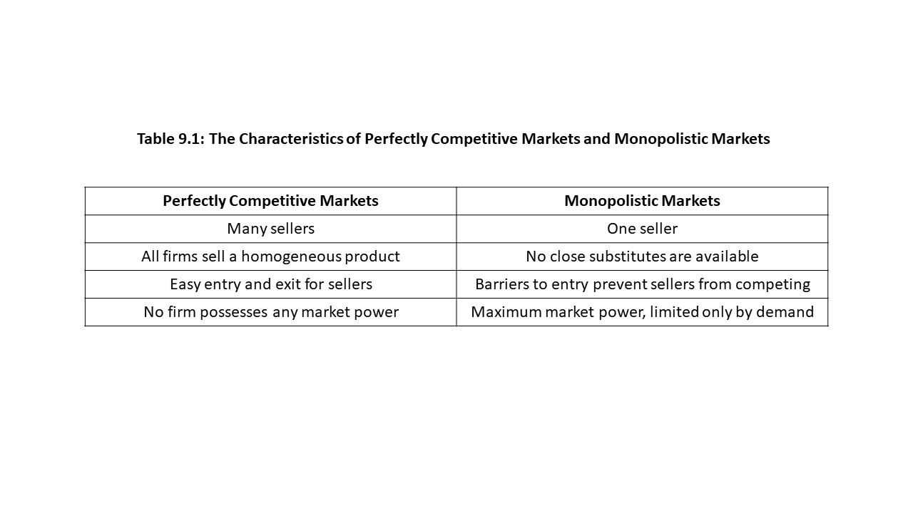
Table 9.1 summarizes the differences between the perfectly competitive market and the monopolist market.
We need to explore the types of entry barriers that make monopolistic markets possible. Often the barriers are legal in nature. Legal barriers to entry include copyrights, patents, licenses, and the ownership of key inputs. We discuss each in turn.
A copyright refers to the exclusive right to reproduce materials (e.g., books, journals, magazines, musical recordings). Since 2003, copyright protection in the United States has been active during the life of the author plus 70 years. One widely cited example of copyright protection is Time Warner’s ownership of the copyright to the song “Happy Birthday.” As of 2004, Time Warner was earning about $2 million per year in royalties due to its ownership of this copyright.[1] It is the reason that the employees in many restaurants sing different songs rather than the song “Happy Birthday” to their customers when they learn that customers are visiting their restaurants on their birthdays.[2] Any public performance of the song without the payment of royalties to the owner of the copyright exposes the performer to a potential lawsuit. Another famous example is Michael Jackson’s purchase of the copyright to the Beatles’ songs in 1985 for $47.5 million.[3] Although it was a lot of money, the estimated value in 2006 was $1 billion![4]
Patents are another kind of legal barrier to entry. A patent is the exclusive right granted to an inventor to produce and sell a product for a specific period. In the United States, the government grants patent protection for 20-year terms. Patents are particularly important in the pharmaceutical industry in which large corporations develop certain types of drugs and medications and possess the exclusive right to sell them during the term of the patent. The justification for patents and copyrights is that firms and individuals need incentives to incur the costs of developing inventions and creating artistic and professional work. If competitors could immediately duplicate and compete in the sale of the newly invented product or the newly created work, then the creator would not have an opportunity to recoup the costs. The consequence would be a lack of invention and artistic activity in our society. The downside, of course, is that competition in the protected area does not allow the price of the new product or material to decrease. As a result, a tradeoff exists between innovation and low product prices. For this reason, patent and copyright protection have limited terms.
Licenses are another important type of barrier to entry. An occupational license is legal permission to conduct a specific line of business. For example, licenses are required to practice law and medicine. The belief is that some professions provide services that may harm consumers if unqualified individuals practice in those areas. The government uses licensing requirements then as a safeguard against the entry of unqualified service providers. Strictly speaking, we should not regard these markets as monopolistic. Those licensed to practice law jointly hold the monopoly power within the legal profession. Considerable competition exists between the many licensed professionals who sell legal services. The same applies to those who have licenses to practice medicine.
Finally, the ownership and control of key inputs is another legal barrier to entry because it depends on property rights. That is, if a firm has a monopoly in a key resource market, then it also frequently has a monopoly in the product market. For example, the Aluminum Company of America (ALCOA) once had a monopoly in the market for bauxite, which is the critical input to produce aluminum. Its monopoly in the market for bauxite allowed it to monopolize the aluminum market.[5] Similarly, in the late nineteenth century, Standard Oil acquired all the major pipelines for the transportation of oil in the United States helping it to solidify its monopolistic control of the transportation side of the oil business. During this same period, Carnegie Steel acquired a controlling interest in a major producer of coking coal, which the company then used in the production of steel. This acquisition helped Carnegie’s company to dominate the steel market.
Aside from legal barriers to entry, we can also identify one key economic barrier to entry that may lead to the formation of a monopoly market. In Chapter 7, we discussed the concept of economies of scale (EOS). This concept refers to the way in which per unit production cost declines as a firm expands in the long run. This phenomenon occurs for a variety of reasons, including the spreading of large startup costs over many units of output, labor and managerial specialization, and learning by doing. Economies of scale may give one firm such a large economic advantage over its competitors that it is able to completely monopolize a market even in the face of unrestricted competition. When a firm acquires a monopoly due to economies of scale, neoclassical economists refer to it as a natural monopoly.
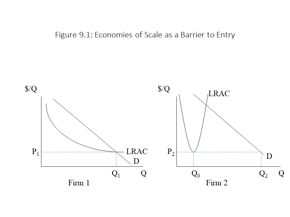
Consider the long run average cost (LRAC) curves of the two firms represented in Figure 9.1.
Firm 1 enjoys considerable economies of scale as can be seen from the falling LRAC over a large range of output. Firm 2, on the other hand, experiences diseconomies of scale at relatively low output levels as indicated by the rapid increase in LRAC even while the firm is operating at a very low output level. The market demand is similar in each market. If Firm 1 charges a low price (P1) that just allows it to cover the minimum LRAC, then its production at the minimum efficient scale (MES) is sufficient to meet the entire quantity demanded in the market (Q1) at that price. The situation is different with Firm 2 if it also sets a price (P2) that just allows it to cover the minimum LRAC. Firm 2 will produce at MES, but this quantity (Q0) is not nearly enough to supply the entire quantity demanded in the market (Q2) at that low price.
In this case, Firm 1 is the natural monopoly. The reason is that if multiple firms with the same LRAC curve were to produce only a fraction of the output, then the LRAC for each firm would be much higher than it is when a single firm produces for the entire market. A single firm in that case is the most efficient outcome from a cost-minimizing perspective, and the scale economies of the firm serve as a barrier to entry keeping out potential competition. On the other hand, if multiple firms produce in the industry in which Firm 2 operates, these firms can collectively produce enough to satisfy the entire quantity demanded in the market even as each produces at the MES. In that case, the most efficient outcome is to have multiple firms competing with one another, and this industry is not one in which a natural monopoly is likely to operate.
The Nature of Demand and Marginal Revenuein Neoclassical Monopoly Theory
We are now to the point where we can begin to analyze the neoclassical theory of monopoly markets. We begin by considering the demand curve facing the monopolist. Because the monopolist is the only seller in the market, the monopolist faces the entire market demand curve. Furthermore, this demand curve that the monopolist faces is likely to be relatively inelastic. The reason is that no close substitutes for this product exist, and we learned in Chapter 5 that the availability of substitutes is a major determinant of the price elasticity of demand. When no close substitutes are available, consumers become much less responsive to changes in the price of the product. This aspect of the market demand curve in a monopoly market strengthens the market power of the monopolist.
For the sake of comparison, we should consider how the demand curve facing the monopolist differs from the demand curve facing the perfectly competitive firm. Figure 9.2 shows the demand curves facing a monopolist and a perfectly competitive firm.
The perfectly competitive firm faces a horizontal demand curve because the firm is small and only faces a segment of the market demand. As explained in Chapter 8, a perfectly competitive firm is a price-taker for this reason. Consumers are perfectly responsive to price changes and so demand is perfectly elastic.
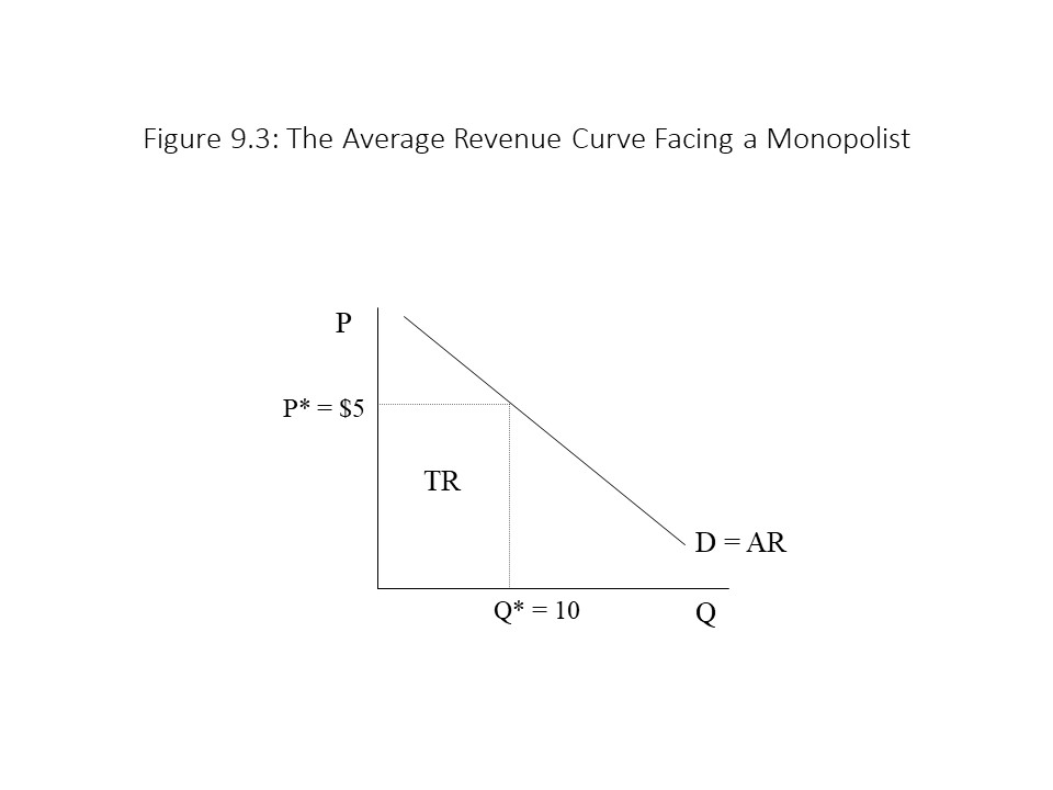
As when we investigated the revenue structure of the perfectly competitive firm, we will now consider the revenue structure facing the monopolist. It is assumed at this stage that the monopolist charges the same price for every unit sold. As a result, the firm’s total revenue (TR) may be represented in Figure 9.3 when the price charged is $5 per unit and the quantity demanded is 10 units.
Clearly, the firm’s TR in this case is $50 (= $5 per unit times 10 units) and is represented as the area of the rectangle in the graph. The average revenue (AR) can also be calculated as follows:
It turns out that the AR in this case is the same as the price charged. This result will generally hold as can be seen below:
What this result implies is that at any level of output, we only need to look at the height of the demand curve to obtain the firm’s AR just as we look at the height of the demand curve to obtain the price at that output level. Therefore, the demand curve facing the monopolist is identical to the firm’s AR curve as indicated in Figure 9.3.
It should also be noted at this stage that the monopolist can set the product price or the quantity exchanged, but it cannot choose both variables independently. That is, if the monopolist selects the price, then the consumers will decide which quantity to demand at that price. Similarly, if the monopolist decides that it will sell a specific amount of its product, then the consumers will decide which price they are willing and able to pay to purchase that amount of the product.
We next turn to the monopolist’s TR curve. As the reader might recall from Chapter 5, the TR curve has a specific shape in the case of a downward sloping linear demand curve. It is shown in Figure 9.4.
In Chapter 5, we learned that the reason for this shape is that at high prices demand is elastic and so price cuts lead to larger percentage increases in quantity demanded, which causes TR to rise overall. Once the price falls below the point of unit elasticity, demand becomes inelastic and further price cuts lead to smaller percentage increases in quantity demanded. As a result, TR falls. The pattern of TR as output changes is much more complicated for a monopolist than for a perfectly competitive firm. In the last chapter, we learned that a perfectly competitive firm’s TR rises continuously in a linear fashion because the firm faces a constant price as output rises. In the case of the monopolist, the firm is cutting price to sell additional units of output, and the changing demand elasticity causes TR to rise and then fall.Figure 9.5 and that we know two points on the market demand curve.
In Figure 9.5, the price falls from $6 per unit to $5 per unit, and the quantity demanded subsequently rises from 3 units to 4 units. The TR increases from $18 to $20 indicating that the firm is selling in the elastic portion of the market demand curve. The MR of the fourth unit of output may be calculated as follows:
In other words, the firm’s TR only rises by $2 due to the increase in output from 3 to 4 units. This result might seem surprising, especially given the fact that the fourth unit of output sells at a price of $5! What is the reason for this strange result? While it is true that the fourth unit sells at a price of $5, it was necessary to reduce the price from $6 to $5 for every unit sold to sell that fourth unit. Therefore, the firm gains $5 in additional revenue from the sale of the fourth unit even as it loses $3 due to the price cut (i.e., $1 for each of the three units previously sold at a price of $6 each). The net change in revenue is $2 (= 5 – 3). The implication then is that the MR of the fourth unit is below the price of the fourth unit. This point is indicated in Figure 9.5 where the MR2 is equal to $2 and the quantity of output is 4 units. Because the MR is generally less than the price of the product, we can draw the MR curve as a downward sloping curve that falls faster than the demand curve, as shown in Figure 9.5.
We have just seen that the MR curve for a monopolist falls faster than the demand curve facing the monopolist because the firm must reduce the price on all units sold when it wishes to sell an additional unit. It is helpful to contrast the MR curve facing the monopolist with the MR curve facing the perfectly competitive firm. If the perfectly competitive firm faces a constant market price of $5 per unit, then we can calculate the firm’s MR as shown in Figure 9.6.
Using the information in Figure 9.6, we can see that the MR is calculated as follows:
Without the need to reduce price to sell an additional unit, the perfectly competitive firm’s MR is the same as the price charged.
We can also understand the shape of the MR curve facing the monopolist from a mathematical perspective if we consider the relationship between MR and TR. The MR is defined as ΔTR/ΔQ. If we consider the TR curve facing the monopolist, then we can see that the MR is nothing more than the slope of the TR curve. As Figure 9.7 shows, the slope of the TR curve at a given output level can be determined using the tangent line method.
It should be clear that in the elastic portion of the demand curve, the MR is positive because the slope of the TR curve is positive. Similarly, at the peak of the TR curve where demand is unit elastic, the MR is equal to zero because the slope of the TR curve is zero. Finally, in the inelastic portion of the demand curve where the TR is falling, the MR must be negative because the slope of the TR curve is negative.
We can also infer at this stage that the monopolist will never produce where demand is inelastic. If the monopolist produces in this region of the demand curve then MR will be negative, which means that TR will be falling. A firm can never increase its economic profits by producing in this region because its TR will be falling even as its total cost (TC) is rising due to the increase in production. At this stage, we have not even incorporated TC into the analysis of the pure monopolist, but it is certain that higher production increases TC. As a result, economic profit must fall if the firm produces where demand is inelastic. Therefore, the monopolist will only produce where MR is greater than or equal to zero. This result tells us that a monopolist will tend to produce relatively less output rather than more, but at this stage, we cannot draw a more precise conclusion about the profit-maximizing choice of the monopolist.
Short Run Profit Maximization: Rules and Cases
Now that we have fully explored the revenue structure of the pure monopolist, we can turn to the question of profit-maximization. That is, which output level will be chosen and which price will be charged to maximize the firm’s economic profit in the short run? To answer this question, we must introduce production cost into the analysis. We will assume that the cost structure facing the pure monopolist is identical to the cost structure elaborated in Chapter 7 and applied to the perfectly competitive firm in Chapter 8. It also turns out that the two rules of profit maximization in the short run that were applied in the case of a perfectly competitive firm are also applicable in the case of the purely monopolistic firm. That is:
The firm should produce where MR=MC.
The firm should only produce a positive output level when P≥AVC.
Table 9.2 provides detailed information facing a monopolistic firm.
The first two columns contain given information about the market demand schedule that the firm faces. Clearly, the market demand curve is downward sloping. TR is calculated as the product of price and quantity demanded in the market. MR is calculated in a manner just like that described earlier in this section. For example, we calculate the MR of the 20th unit of output as follows:
The TC information in Table 9.2 is given, and the ATC, MC, and economic profit (π) calculations are all carried out as in earlier chapters.
A few details from Table 9.2 deserve special emphasis. The TR peaks at 60 units of output. At higher output levels, TR begins to fall and MR becomes negative. We can infer that demand becomes inelastic beyond 60 units of output. Because we are using discrete data for the level of output (e.g., 0, 10, 20, …), the MR is close to zero but not exactly equal to zero when the TR reaches its peak. As a result, we know that the firm must produce 60 units of output or less to maximize its economic profit since those output levels correspond to the elastic part of the demand curve. To be more precise, we can now apply the rule that the firm will produce where MR = MC (if P ≥ AVC). In the table, MR and MC are equal to $6 per unit at an output level of 50 units. We do not have specific information for AVC in the table, but since P > ATC at 50 units of output, P must necessarily exceed AVC. The firm earns its maximum economic profit of $300 at 50 units of output. It might be noticed that 40 units of output will also achieve this same amount of economic profit. Again, it is our use of discrete data that is responsible for this result, and so it is always best to focus on the rule that MR = MC.
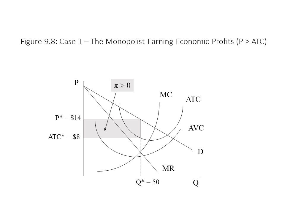
Figure 9.8 shows how the monopolist’s situation appears graphically.
It is important to notice that even though the profit-maximizing output level is found directly below the MR = MC intersection, the profit-maximizing price that is charged is found above the intersection on the market demand curve. The area of the shaded box represents the firm’s economic profit of $300, which may be calculated as the product of the amount by which P exceeds ATC (= $6 per unit) and the quantity sold (= 50 units). Alternatively, TR is $700 (= $14 per unit times 50 units) and TC is $400 (= $8 per unit times 50 units). The economic profit of $300 is simply the difference between the two amounts.
This analysis demonstrates that the goal of the monopolist is not to rip off the consumer. The monopolist aims to maximize economic profit. It could charge the consumer a higher price if it wished to do so, but a higher price would reduce its economic profit. We know that economic profit would be lost because at a higher price, the firm’s MR exceeds its MC. Similarly, the firm could increase the quantity sold by reducing its price, but this action too would fail to maximize economic profit because a lower price would cause MC to exceed MR.
It is worth emphasizing that the monopolist does not have a supply curve like the perfectly competitive firm.[6] As we learned in Chapter 8, the perfectly competitive firm’s profit-maximizing quantity changes as the market price changes for reasons beyond the firm’s control. As the market price changes, we observe different quantities supplied by the perfectly competitive firm at each price. The monopolist, on the other hand, chooses the market price to maximize its economic profit. As a result, the price charged does not fluctuate for reasons beyond the monopolistic firm’s control. Therefore, the only relevant combination of output and price for a monopolist is the one that it chooses to maximize its economic profit. It is not possible to trace out a series of combinations of price and quantity supplied in the case of the monopolist.
In addition, the economic profits that the monopolist earns may persist even in the long run due to the barriers to entry that prevent competitors from entering the market.[7] In the case of perfect competition, economic profits serve as a signal to firms outside the industry to enter. The lack of entry barriers leads to a rise in the market supply and a reduction in the market price until the economic profits are eliminated. No such elimination of the economic profits can occur in the case of pure monopoly. Although the monopolist is protected from competition, its economic profits are not guaranteed. If consumer demand falls then the market demand curve will shift to the left, which may eliminate the economic profits.[8] Similarly, a rise in production costs may occur, which would cause the ATC curve to shift upwards.[9] The result again would be a reduction in economic profits.
These possibilities lead us to consider additional scenarios that may face the monopolist in the short run. Figure 9.9 represents the case where a monopolist is operating at the break-even point.
In Figure 9.9, the firm maximizes its economic profit by producing 45 units of output. This output level corresponds to the MR = MC intersection, and the price of $12 per unit at this output level is clearly above AVC. In fact, at Q = 45 units, the price equals the ATC. As a result, the firm’s TR is $540 (= $12 per unit times 45 units) and the firm’s TC is $540 (= $12 per unit times 45 units). Its economic profit is, therefore, equal to zero and so it is not represented as a shaded area in the graph. It should be recalled that this situation is acceptable to the monopolist because the firm is covering all its costs, including the opportunity cost of producing in this industry. Greater economic profits are always desired, of course.Figure 9.10 shows another scenario in which the monopolist maximizes its economic profit by producing 42 units of output.At that output level, MR = MC but also the profit-maximizing price of $10 is above the AVC of $6. The firm’s TR in this case is $420 (= $10 per unit times 42 units), and the firm’s TC is equal to $504 (= $12 per unit times 42 units). The economic profit then is equal to -$84 (= $420 – $504), which is also equal to the area of the top shaded box in Figure 9.10. If the firm is suffering a loss as indicated by its negative profit, then why does the firm operate in the short run? The reason is that the loss from shutting down would be even larger. As we discussed in Chapter 8, whenever a firm shuts down in the short run, its economic profit is equal to –TFC. The TFC can be calculated as the product of the AFC and the level of output. In this case, the TFC is equal to $252 (= $6 per unit times 42 units), which is also equal to the combined area of the two shaded regions in Figure 9.10. Clearly, an economic profit of -$252 is much worse for the firm than an economic profit of -$84. Therefore, the monopolist will choose to operate in the short run at a loss.Figure 9.11.
In this case, the firm charges a profit-maximizing price of $8 per unit, which is also equal to the firm’s AVC at this output level. Because the shutdown rule states that the firm will produce where MR = MC if P is greater than or equal to AVC, we conclude that the firm will operate in this case. The firm’s TR in this scenario is equal to $296 (= $8 per unit times 37 units). The firm’s TC is equal to $518 (= $14 per unit times 37 units). Therefore, the economic profit is equal to -$222. In addition, the firm’s TFC is equal to $222, which may be calculated as the product of AFC (= $6) and Q (= 37 units). Therefore, if the firm shuts down, it will suffer an economic loss of $222 (= -TFC), which is exactly equal to its loss from operating. In Figure 9.11, the shaded region represents both the TFC and the economic loss from operating. Even though the firm is indifferent between operating and shutting down, we conclude that the firm operates.
Another way to argue that the firm is indifferent between operating and shutting down is to note that the firm is earning just enough revenue to cover its TVC. The firm’s TVC is equal to $296 because TVC may be calculated as the product of AVC (= $8) and Q (= 37 units). In other words, the firm can just pay wages out of revenue so it is only the TFC that it cannot cover when it operates.
The final case that we will consider for the short run is the case in which the monopolist decides to shut down as shown in Figure 9.12.
In this case, the firm produces no output because the price of $6 per unit, which is directly above the MR = MC intersection, is below the AVC of $7 per unit. Because the monopolist shuts down, its TR is $0 and its TVC is $0. It must still pay its TFC and so its economic profit is equal to –TFC. As always, the TFC may be calculated as the product of AFC and Q, which is here equal to $272 (= $8 per unit times 34 units). The firm’s economic loss of $272 is depicted as the top shaded box in Figure 9.12. If the firm were to produce 34 units and charge a price of $6 per unit, then its economic loss would be much greater. In that case, the monopolist’s TR would be $204 (= $6 per unit times 34 units), its TC would be $510 (= $15 per unit times 34 units), and its economic profit would be -$306 (= $204 – $510). The economic loss in that case would be equal to the combined area of the two shaded boxes in Figure 9.12. As a result, the firm opts to shut down and limit its losses to the TFC.
Implications for Efficiency and the Long Run
The five cases that we considered in the previous section are all possible scenarios that the monopolist will face in the short run. As we observed, it is only in cases 1-4 that the monopolist will operate in the short run. Whenever price falls below AVC, as in case 5, the firm shuts down. The reader might wonder which of these cases is possible in the long run. In the long run, the firm will withdraw its capital and exit the industry if it is experiencing economic losses. Cases 3-5 all include economic losses and so these cases cannot apply to the monopolist in the long run. On the other hand, cases 1 and 2 involve an economic profit that is greater than or equal to zero. As we have seen, an economic profit of zero will be acceptable even to a monopolist in the long run because all costs are being covered, including opportunity costs. Furthermore, we have seen that barriers to entry make long run economic profits a real possibility because competitors cannot enter and drive down the price. Therefore, either of these two cases is a possible long run equilibrium.
Our next task is to consider the efficiency implications of monopoly markets. We have seen that perfectly competitive markets achieve economic efficiency in the sense that they lead to least-cost production (productive efficiency) and the appropriate quantity of the good produced (allocative efficiency). They also maximize the total of consumer surplus and producer surplus. It is worth asking whether monopoly markets achieve the same desirable outcomes.
Figure 9.13 allows us to compare the efficiency effects for the cases of pure monopoly and perfect competition.
In Chapter 8, we learned that the marginal cost (MC) curve of a perfectly competitive firm is the same as the perfectly competitive firm’s supply curve (for MC above minimum AVC). It followed that the aggregation of the MC curves of all the perfectly competitive firms in the industry would yield the market supply curve. If we assume that the monopolist operates with the same production technology as the perfectly competitive firms, then we can assume that the monopolist’s MC curve is identical to the market supply curve that would emerge if the market was perfectly competitive. For this reason, the monopolist’s MC curve in Figure 9.13 is also labeled as a perfectly competitive market supply curve (= S). This approach allows us to compare the efficiency effects of the two market structures on the same graph.Figure 9.13. If the market is monopolistic, on the other hand, then the monopolist produces Qm where MR and MC intersect and charges a price of Pm as shown on the market demand curve above that point. Clearly, the monopolist produces a smaller quantity and sells it at a higher price than would emerge in a perfectly competitive market. The failure to produce where marginal benefit (represented by demand) and marginal cost intersect indicates that the monopoly market does not achieve allocative efficiency. Indeed, this result is the main reason that neoclassical economists object to monopoly markets. Unlike consumers who tend to complain about high monopoly prices, neoclassical economists tend to focus much more on the fact that monopolies do not produce as much of the product as would be produced in a perfectly competitive market.
The monopoly firm also fails to achieve least-cost production. If we look back at Figure 9.8, for example, in which the firm is enjoying economic profits, we can see that the price charged is clearly above the minimum ATC, which exists at the intersection of MC and ATC. If the firm was to produce more, then its ATC would fall due to further specialization within its production plant. It chooses not to expand production, however, because holding back production allows the firm to raise the price by more than enough to make up for the higher unit cost.
Returning to Figure 9.13, we can also see that the reduction in output that occurs in the monopoly market leads to a loss of consumer surplus and producer surplus. The reader should recall that the consumer surplus is equal to the area above the current price and below the demand curve. In this case, the increase in price that the monopolist pursues causes the consumer surplus to shrink by the amount of the shaded rectangle and the top shaded triangle. The top shaded triangle, however, represents a pure loss to society because it corresponds to the reduction in quantity that accompanies the monopolization of the market. These units are not produced anymore and so this consumer surplus is completely lost. The shaded rectangle, however, corresponds to units that are still produced in the monopoly market. This area represents a transfer to the producers in the form of producer surplus. For this reason, the shaded rectangle is referred to as the rectangle of redistribution. These units are still sold but now at the higher monopoly price.
The reader should recall that producer surplus is represented as the area below the current price and above the supply curve (or the marginal cost curve). The reduction in output that occurs with the monopolization of the market thus leads to the loss of the bottom shaded triangle in Figure 9.13. Because these units of output are no longer produced, this producer surplus is simply lost. This loss of producer surplus, of course, raises the question as to why the monopolist would restrict output when it leads to a loss of producer surplus. The reason is that this reduction in output makes possible a rise in price, which allows the monopolist to capture a significant part of the consumer surplus. A net gain for the monopolist is the result.
What happens in this case is that the total surplus (TS) that society realizes shrinks due to the loss of consumer surplus and producer surplus. This loss of TS represents an efficiency loss from the monopolization of the market. The two shaded triangles in the graph represent the deadweight loss of monopoly. The larger triangle formed from the combination of these two smaller triangles is called a Harberger Triangle after the American economist Arnold Harberger for whom it is named. In summary, the total economic pie shrinks due to the monopolization of the market even as the monopolist grabs a larger share for itself at the expense of consumers.
Additional characteristics of monopoly markets also strengthen the case that such markets tend to be inefficient. Specifically, monopolistic firms have an incentive to incur additional costs to maintain the barriers to entry that keep competitors out of their markets. Firms may hire lobbyists to pressure lawmakers to extend their patents and copyright protection. Lawyers may be hired to initiate lawsuits against those believed to be infringing on the firm’s rights of ownership of patents and copyrights. Because these expenses are incurred to protect the firm’s economic profits rather than to increase production, they are regarded as wasteful from a social perspective. Neoclassical economists label these efforts to appropriate benefits that exceed the economic cost of the required resources as rent-seeking activities. To the extent that these legal barriers to entry encourage innovation, that benefit may provide some economic justification for these expenses. Any costs that exceed what is needed to encourage innovation, however, are regarded as socially wasteful in neoclassical theory.
In terms of long run economic growth, monopolies are also often accused of being technologically backwards.[10] That is, because they are not subject to competitive pressure, the claim is made that they will not have the incentive to innovate and keep production costs down in the same way that a perfectly competitive firm would. An example of a large firm that lost considerable market share due to a failure to innovate is General Motors. Although it was not a pure monopoly in the American automobile market given the presence of other large automakers, it was the market leader in the mid-twentieth century. Its failure to keep up with market trends caused it to lose considerable market share to Japanese auto producers as Japanese auto companies began selling smaller, more fuel-efficient cars in response to the rise in gas prices in the 1970s. Another interesting example of the tendency of large corporations to stagnate technologically is U.S. Steel’s refusal to develop a new steel beam known as a Grey beam at the beginning of the twentieth century. By 1926, U.S. Steel was secretly producing the Grey beam in violation of Bethlehem Steel’s patent rights. Eventually, U.S. Steel was forced to pay royalties to Bethlehem Steel in exchange for permission to produce the Grey beam.[11]
Natural Monopoly and Price Discriminating Monopoly
Overall, monopolies appear to be economically inefficient. Nevertheless, we can identify some exceptions to this general rule. One example is when a natural monopoly exists. As we have seen, natural monopolists enjoy an economic cost advantage due to economies of scale. It is this cost advantage that allows them to dominate the market. If significant economies of scale exist in an industry, then our assumption breaks down that the MC of the monopolist is the same as the market supply curve in a perfectly competitive market. With significantly lower per unit production costs, the natural monopolist may end up being more efficient than the perfectly competitive market.
As we discussed earlier in this chapter, a natural monopolist enjoys falling LRAC over a large range of output. Public utilities are frequently cited examples of natural monopolies. The startup costs are very large and so these costs are spread out over a large quantity of output. Most areas are served by a single electric company, a single natural gas company, and a single water company. Imagine the inefficiencies that would arise if many suppliers each had their own electrical wires, gas lines, and water delivery systems. Consider the case of an electric company that enjoys large economies of scale in production and so monopolizes the local electricity market. This case is depicted in Figure 9.14.
In Figure 9.14, the quantity of output is measured in millions of kilowatt hours (kwh) used per month. The price and unit costs are measured in dollars per kilowatt hour. Economies of scale are clearly present as can be seen from the declining LRMC and LRAC curves. The monopolist also faces a downward sloping demand curve and has a corresponding MR curve that declines more quickly than price. If the monopolist is allowed to operate freely, it will maximize its economic profit by selling 20 million kwh at a price of $0.20 per kwh. Because the monopoly price (PM) exceeds LRAC at 20 million kwh, clearly the monopolist will earn an economic profit.Figure 9.14. One possibility is to require the electricity provider to charge a price equal to LRMC ($0.05 per kwh in this example) as is the case in a perfectly competitive market in long run equilibrium. This regulatory strategy is known as marginal cost pricing. If the firm is also required to produce the perfectly competitive level of output of 29 million kwh, then the price is much lower and the quantity sold is much higher than in the profit-maximizing outcome. The problem is that the regulatory board has forced the monopolist to suffer losses as indicated by the fact that the price charged is below LRAC at that output level.
An alternative regulatory strategy is to require the monopolist to charge a price equal to LRAC. This regulatory strategy is known as average cost pricing and guarantees that the firm will earn an economic profit of zero. If the firm charges a price of $0.10 per kwh and produces an output level of 25 million kwh, then the firm will break even. This pricing rule leads to a larger quantity of output sold than in the monopoly outcome but not as much as the marginal cost pricing rule. It also leads to a lower price than the monopoly price but one that is higher than the perfectly competitive price. It thus represents a compromise between the two possible outcomes that is still acceptable to the natural monopolist, even in the long run since economic profits are zero.
Another possible scenario in which a monopolist may be more efficient than the basic model occurs when the monopolist can engage in price discrimination. Price discrimination refers to the practice of charging different prices to different consumers of the same product. For example, student discounts on restaurant meals or movie tickets are good examples of price discrimination. Regular customers must pay full price but the students are given a discount to encourage them to patronize specific establishments. Senior discounts on restaurant meals and kids’ menus are other examples. Additional examples include bulk discounts. When a consumer buys a 24-pack of soda, for example, she will generally pay a lower price per can than if she purchases a 6-pack of soda.
The examples of price discrimination cited above involve different groups of consumers being charged different prices based on some distinguishing characteristic of the consumer or the quantity that is purchased. The purest form of price discrimination, however, occurs when every consumer in a market is charged the maximum price she is willing and able to pay. This form of price discrimination is referred to as perfect price discrimination because it is only possible when the seller can perfectly discriminate between consumers. For this form of price discrimination to occur, the firm must be a monopolist. If competitors can charge lower prices than the maximum that the consumers are willing and able to pay, then this pricing strategy will be undermined very quickly. The monopolist must also have complete knowledge of the market demand curve. Otherwise, it will be impossible to identify the maximum prices that consumers are willing and able to pay. Finally, it must be impossible for consumers to resell the units they purchase.[12] If a consumer who is willing and able to pay a low price can turn around and sell that unit to a consumer who is willing and able to pay a much higher price, then the monopolist may fail to make the sale to the consumer who is willing and able to pay the high price, particularly if the consumer who resells the unit charges a slightly lower price for that unit.
Figure 9.15 shows the case of a monopolist that is capable of perfect price discrimination.[13]
The major difference between this graph and the graph of the single pricing monopolist is that this monopolist’s MR curve is identical to the demand curve facing the firm. With a single pricing monopolist, the MR curve is steeper than the demand curve because the firm must cut the price on all units sold to sell another unit. When the monopolist can perfectly price discriminate, however, it does not need to cut the price on other units sold to sell one additional unit. As a result, the MR of an additional unit is the same as the price. Therefore, the market demand curve and the MR curve are the same in the case of perfect price discrimination. In Figure 9.15, the first unit is sold for $9 per unit, which is the maximum price that a consumer is willing and able to pay for that unit. The second unit sells for $8. Notice that the first unit still sells for $9 even though the second unit sells for $8 because perfect price discrimination occurs in this case. The MR of the second unit then is $8 because TR rises by the full amount of the price of that unit. The third, fourth, and fifth units sell for $7, $6, and $5, respectively. Notice that the monopolist will stop producing at 5 units because at this point MR = MC. The firm’s TR is calculated as the sum of the different prices charged as follows:
The monopolist’s total cost is calculated as it always is. If we multiply the ATC at the profit-maximizing output by the quantity produced, then the TC is equal to $20 (= $4 per unit times 5 units). The firm’s economic profit then is equal to $15 (= $35 – $20).
Because the perfectly price discriminating monopolist can charge the maximum price the consumer is willing and able to pay, the firm appropriates the consumer surplus that consumers normally enjoy when they pay the single market price. This transfer to the monopolist allows the monopolist to increase its economic profit at the expense of the consumer. This result is important because it demonstrates that price discrimination is not a practice that is adopted to help special groups like senior citizens, parents with small children, and college students. The practice is adopted because it maximizes economic profits. By charging lower prices to senior citizens and kids and higher prices to everyone else, a restaurant can appropriate (at least in part) the smaller consumer surpluses of the senior citizens and children and the larger consumer surpluses of everyone else.
We can also see that a perfectly price discriminating monopolist is more efficient than a single pricing monopolist. Specifically, if we assume once more that the MC curve of the monopolist is the same as the market supply curve if the market was instead perfectly competitive, then we can evaluate the efficiency effects of price discriminating monopoly relative to perfect competition. In Figure 9.15, the perfectly competitive equilibrium can be found at the intersection of the market demand curve and the MC curve of the monopolist (i.e., the perfectly competitive supply curve). The perfectly competitive output level is 5 units of output, which is the same as the profit-maximizing output of the price discriminating monopolist. In other words, the price discriminating monopolist achieves allocative efficiency. It fails, however, to achieve least-cost production because the ATC of $4 per unit is above the minimum ATC, which occurs at the intersection of the ATC and MC curves. The implication is that perfect price discrimination does not shrink the economic pie, but it does redistribute a large part of the pie away from consumers and towards the monopolist.
Government PolicyRegardingMonopoly
Because monopolists tend to operate inefficiently, the question arises as to how society should respond when monopolistic markets emerge. We can identify five possible responses. Each response may be associated with a specific school or schools of economic thought.
The Austrian and Randian perspectives: Allow private monopolies to thrive without government intervention.
The conservative neoclassical perspective: Divide inefficient monopolies into competing firms by enforcing antitrust laws.
The liberal neoclassical perspective: Publicly regulate privately owned natural monopolies and divide monopolies into competing firms with even stricter enforcement of antitrust laws.
The statist perspective: Create public monopolies through nationalization (state acquisition)
The traditional socialist perspective: Grant the power to bodies of working people to cooperatively plan production in monopoly firms in coordination with other bodies of working people and consumers.
We can place each of these views along the political spectrum ranging from far right to far left as shown in Figure 9.16.
We will briefly discuss each of these responses beginning with the neoclassical perspectives since we have already explored the neoclassical theory of monopoly in detail. According to conservative neoclassical economists, the ideal market structure is the perfectly competitive one. Therefore, efficiency can be enhanced by breaking up monopolies into competing firms, effectively transforming a monopolistic market structure into a perfectly competitive market structure. The notion that government intervention can be used to create a more competitive environment is one that has a long history in the United States. The 1890 Sherman Act was the first major piece of federal legislation to outlaw unreasonable restraints of trade. In the early twentieth century, federal action was taken against Standard Oil, U.S. Steel, American Tobacco, and other firms because they had allegedly established illegal monopolies in their industries. The Clayton Act of 1914 and the creation of the Federal Trade Commission (FTC) that same year to enforce the nation’s antitrust laws further strengthened this instrument of federal control over markets. The conservative neoclassical perspective takes seriously the benefits of perfect competition, but its proponents prefer that this federal tool be used conservatively (i.e., only when a clear and convincing case can be made that a monopoly is firmly established in a specific industry and is harming consumers).
The liberal neoclassical perspective advocates even stricter enforcement of the nation’s antitrust laws as well as public regulation of privately owned natural monopolies. Again, the aim is to force the natural monopolist to produce a larger output and charge a lower price than its profit-maximizing choices of these variables. In theory, successful regulation using average cost pricing or marginal cost pricing rules will move the industry closer to the perfectly competitive outcome. Conservative neoclassical economists tend to object to regulation because regulatory boards are susceptible to regulatory capture.[14] That is, these boards may come under the influence of the monopolist itself, which can use the coercive power of government to impose its will, thereby creating an even worse situation than that which exists in an unregulated environment. In addition to their advocacy of public regulation of monopolies, liberal neoclassical economists have a lower threshold at which point they advocate antitrust action against potential violators. The remaining perspectives on responses to monopoly are discussed in the next two sections.
The Austrian and Randian Critiquesof Neoclassical Monopoly Theory
The Austrian and Randian perspectives of monopoly theory and antitrust laws are similar and so have been treated together. Differences do exist among adherents of these worldviews, but their commonalities are much greater than the differences. The former chairman of the Federal Reserve Board, Alan Greenspan, was once a member of Ayn Rand’s inner circle. His perspective on U.S. antitrust laws represents the Randian perspective quite well.[15] Specifically, Greenspan challenges the conventional view of the western railroad monopolies that operated in the late nineteenth century. The western railroads have been accused of operating independently of competition even though many were poorly built. Greenspan argues, however, that their monopoly power derived from government subsidies and government restrictions.
According to this Randian perspective, if a single firm becomes dominant in an industry, that fact alone is not reason enough to oppose its existence. Assuming its dominance is the result of its own efficient operation and competitors are free to enter the industry and compete, then the monopolist should not be punished for its success. The only objectionable monopoly, according to this view, is a coercive monopoly. A coercive monopoly is one that maintains its dominance due to legal restrictions that prevent competitors from entering. Once such restrictions are removed, a free capital market will ensure that competitors will enter the industry if they expect that they can compete with the monopolist, argues Greenspan. If the monopolist remains the dominant firm even in the presence of a free capital market, then it will not necessarily have its profits reduced. If the firm is highly efficient and keeps production costs low, then its profit margins may be large. Greenspan argues that a free capital market only ensures that a monopolist that earns big profits by charging high prices will soon face competition that drives those profits down. He identifies ALCOA as an example of a monopoly firm that maintained its monopoly in the market for aluminum for many years prior to World War II due to cost-cutting and efficiency rather than high prices. This opinion contrasts with our earlier suggestion that ALCOA’s control of a key resource was the source of its market power. In summary, a monopolist should never be punished when it achieves and maintains its dominance in an environment of free competition and voluntary exchange.
The Austrian critique of neoclassical monopoly theory resembles the Randian critique. D.T. Armentano, for example, explains that neoclassical economists have placed great emphasis on non-legal barriers to entry like economies of scale and commercially successful product differentiation as sources of monopoly power.[16] Examples of product differentiation include the annual models of automobile companies. Armentano explains that consumers clearly prefer to pay the higher prices that accompany such differentiation. Similarly, consumers could pay the higher prices of firms that do not enjoy scale economies if they wished to do so. From the consumer’s perspective, resources are allocated efficiently and so to use antitrust laws against such firms is in complete opposition to the wills of consumers. Armentano also warns against evaluating the efficiency of monopoly markets against the neoclassical model of perfect competition. He explains that the perfectly competitive model is completely static (i.e., devoid of time and process). As a result, all the features of actual competition, such as product differentiation, advertising, price discrimination, and innovation, are treated as monopolistic practices that lead to the misallocation of resources. If we regard all such activities as monopolistic, then most competitive interaction will be viewed as requiring government intervention, in Armentano’s view.
Along similar lines, Armentano explains how the Austrian economist Murray Rothbard argues that it is not possible to conceptually distinguish between a monopoly price and a free market competitive price. If we compare the price of a good in a competitive market with the price of a good in a monopolistic market, then we are simply comparing the prices of two different goods. If consumers are willing to pay a higher price for one of the goods, then the price paid is consistent with the supply and demand for that good just as the lower price is consistent with the supply and demand for that good. Additionally, if the market price of a good rises over time, why should we assume that the initial price is the competitive price and the new price is a monopolistic one? All free market prices ultimately emerge from the interaction of supply and demand and attempts to label some prices as monopoly prices and other prices as competitive prices are simply efforts to justify government interference in the free market.
The Marxian Theory of Monopoly Capital
Marxian economists have also constructed analyses of monopoly capital. These analyses have been complicated, however, by the fact that Marx primarily investigated the conditions of competitive capitalism. Nevertheless, he did recognize the tendency towards monopoly within capitalist industries. One source of this tendency, Marx refers to as the concentration of capital. As an individual enterprise accumulates capital over time, it grows as it devotes a portion of its profits to expansion. The centralization of capital, on the other hand, refers to the tendency of strong, productive enterprises to absorb weaker, less productive enterprises and may be an important factor during capitalist crises. The process is never complete, however, as competition between large capitalists inevitably breaks out again. In Marx’s view, competition gives rise to monopoly and monopoly gives rise to competition.
When Marxian economists have referred to “monopoly capital,” the phrase has been used more generally than the strict neoclassical definition of a single seller in a market for which no close substitutes exist and in which barriers to entry keep competitors from entering. Instead, it seems to refer to industries in which the concentration and centralization of capital have become so great that the law of value no longer prevails. That is, a monopoly capitalist must have the power to increase the price of a commodity above the value that would prevail if the market was intensely competitive. In other words, the monopoly price will be higher than the competitive price that would be charged if the value of the commodity was determined by the SNALT embodied in it. Marxian economists have not put forward an explanation of any economic law that would determine the magnitude of the difference between the monopoly price and the competitive value.
Because of the difficulties associated with the identification of a precise economic law to explain the difference between monopoly price and competitive value, Marxian economists have concentrated more on general qualitative analyses of monopoly capital. The most famous of these analyses is Paul Baran and Paul Sweezy’s Monopoly Capital (1966). Baran and Sweezy argue that over time within capitalist societies a persistent rise in the economic surplus occurs, which is simply the difference between the total social product and the cost of producing it. Because of income inequality, insufficient aggregate demand exists to absorb the surplus. Capitalist consumption and investment are not sufficient to absorb the surplus, and so stagnation is the expected outcome of monopoly capitalism. Some counteracting forces do exist, however, which include the sales effort. The sales effort refers to advertising and product differentiation, which may stimulate demand to a certain degree but which mainly create an enormous amount of waste. Government expenditure is the other major counteracting factor that Baran and Sweezy discuss. Because capitalists have a major influence over government officials, however, they emphasize military expenditures much more than spending on social programs and public assistance because the latter might threaten the class structure of society.[17]
In 2006, John Bellamy Foster and Fred Magdoff argued that the stagnation problem that Baran and Sweezy identified as consistent with the monopoly capital phase had worsened. While the counteracting factors are “superficial, weaker, and self-limiting,” the stagnation tendency is “deeply rooted, powerful, and persistent.” At the same time, Foster and Magdoff argue that the capitalist system has found new ways to offset (at least partly) the stagnation tendency of monopoly capital. They explain that the explosive growth of finance has led to a new hybrid phase of the capitalist system that they refer to as monopoly-finance capital. They explain that the massive growth of finance has led to new outlets for the economic surplus in the finance, insurance, and real estate (FIRE) sectors in the form of new investment in office buildings and equipment. This counteracting factor was limited, however, in that most money capital has been used for speculation in the financial markets rather than for real investment in productive capacity. Due to the inconsistent connection between the financial sector and the industrial sector, the financial explosion has been unable to compensate for the stagnation tendency of monopoly capital enough to revive the rapid accumulation of capital.[18]
Andrew Leigh recently noted that in a recent study involving the examination of thousands of financial reports of U.S. businesses, a 75% reduction in the use of the word “competition” has occurred since the start of the twenty-first century. This lack of interest in competition among U.S. firms suggests that American industry has become increasingly concentrated. Leigh further explains that large corporations charged prices that were 10 to 20 percent above unit costs in the 1980s, whereas now they charge prices that are 60 percent above unit costs. Australia has a similar problem, Leigh argues, because Australian firms have been allowed to merge so that they can more effectively compete in the international marketplace. Leigh recognizes a favorable opinion about large enterprises as consistent with the kind of thinking associated with the Chicago School of Economics. This position, which is very similar to the Objectivist view of monopolies, is that the large corporations possess a large market share because of their superior efficiency. If they raise prices much above their unit production costs, then competitors will enter the market and undermine their monopoly status. As Leigh puts it, large corporations will be “kept in check by the free market.” Leigh also argues that this laissez-faire approach to large firms influenced Australia’s courts and lawmakers, which has led to the increasingly concentrated markets for beer, baby food, insurance, and internet providers. When the government refuses to prosecute firms that behave like monopolies and is willing to approve corporate consolidations, the consequence is a deepening of industrial concentration and enhanced market power. In Australia, for example, Leigh reports that the number of mergers and acquisitions has risen nearly 5 times in the past 25 years. Ultimately, Leigh rejects the automatic acceptance of claims to superior efficiency and wants to shift the focus to the negative impact on consumers through higher prices and on workers through lower wages. When firms cut production below the level that would prevail in a perfectly competitive market, they raise prices to consumers and reduce the amount of labor demanded, which may contribute to wage stagnation.
Summary of Key Points
A monopolist is a single seller in a market for which no close substitutes exist and into which competitors cannot enter due to barriers to entry.
Barriers to entry include copyrights, patents, licenses, ownership of key inputs, and economies of scale.
For a single-pricing monopolist, MR falls faster than price because the firm must cut the price for all units sold to sell another unit.
The profit-maximizing output for the monopolist occurs where MR = MC, and the price charged is set above this output level on the market demand curve.
The monopolist will operate in the short run if the price is at least as great as AVC. The firm will operate in the long run if the price is at least as great as ATC.
Single pricing monopolists fail to achieve allocative efficiency and productive efficiency.
Natural monopolies and perfectly price discriminating monopolies can offset some of the inefficiencies of single pricing monopolies.
The possible government policies to address monopolization range from laissez-faire to outright nationalization or support for worker control.
The only kind of monopoly that is objectionable according to Austrian and Randian thinkers is one that is the product of government entry barriers (i.e., a coercive monopoly).
According to Marxian economists, stagnation is the dominant tendency in the monopoly phase of capitalism, but it is mitigated by the sales effort, government spending, and the expansion of finance.
List of Key Terms
Monopolies
Price-setter
Natural monopoly
Rectangle of redistribution
Harberger triangle
Rent-seeking activities
Marginal cost pricing
Average cost pricing
Price discrimination
Perfect price discrimination
Regulatory capture
Coercive monopoly
Monopoly capital
Concentration of capital
Centralization of capital
Economic surplus
Sales effort
Monopoly-finance capital
Problems for Review
1.Suppose a monopolist reduces the price of its product from $8 per unit to $5 per unit. The quantity demanded of its product subsequently rises from 200 units to 350 units. Calculate the marginal revenue. (Hint: Strictly apply the definition of marginal revenue in this case.) Is the firm operating in the elastic or inelastic portion of the linear demand curve? How do you know?
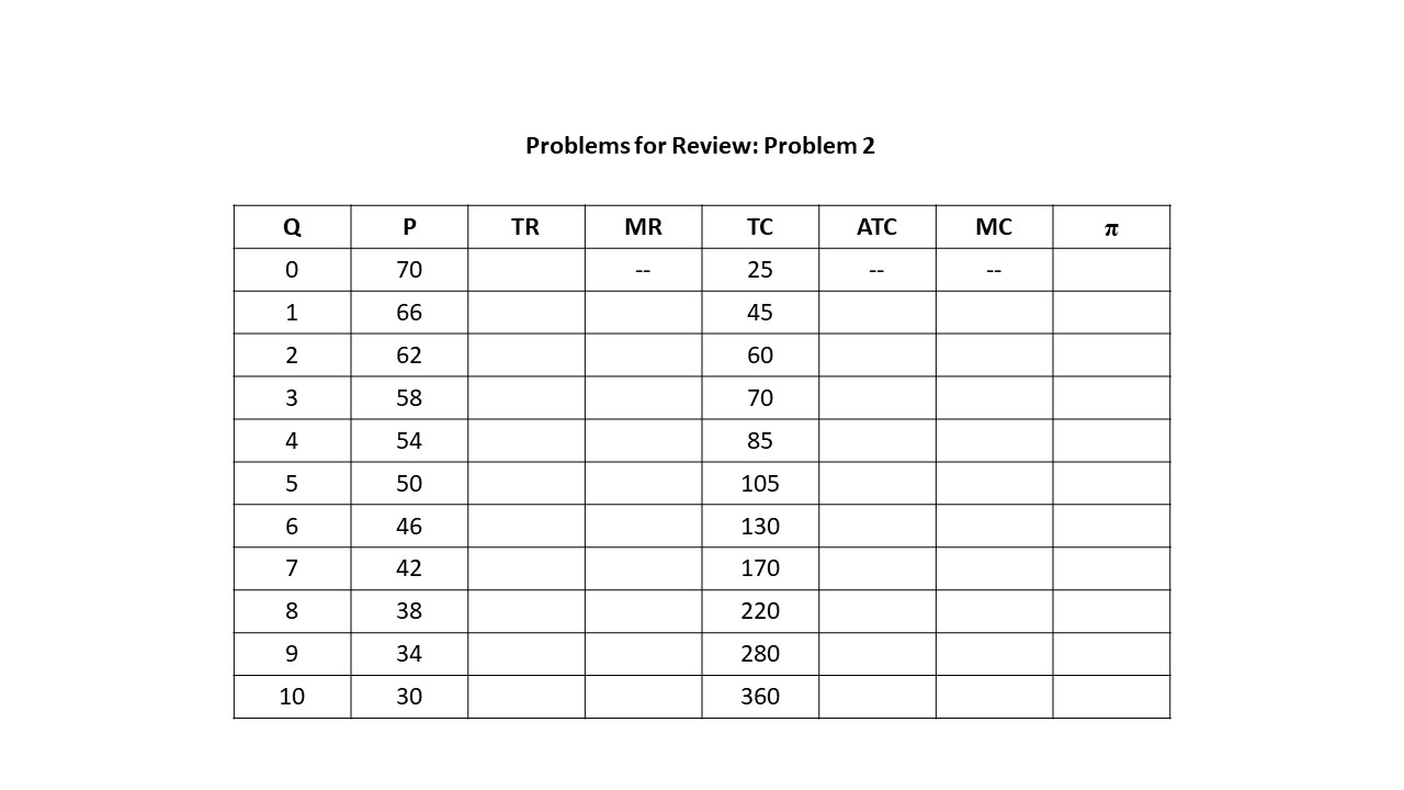
2. The first two columns in the table below represent the demand schedule facing a pure monopolist. Complete the rest of the table using MS Excel.
3. At which output level and price will this monopolist maximize economic profits? How do you know?
4. Create a single graph in MS Excel using the data above that shows the demand curve (D), the marginal revenue curve (MR), the marginal cost curve (MC), and the average total cost curve (ATC). Be sure to label both axes.
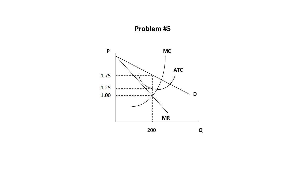
5. Using the graph below, identify the following, assuming the firm maximizes its economic profit in the short run:
Output
Price
Total revenue
Total cost
Economic profit
Will the firm operate in the short run?
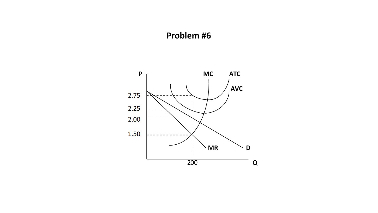
6. Using the graph below, identify the following, assuming the firm maximizes its economic profit in the short run:
This example is a commonly cited example in neoclassical textbooks. See Hubbard and O’Brien (2019), p. 512. ↵
McConnell and Brue (2008), p. 430, offer a graphical method of demonstrating this point. ↵
Bade and Parkin (2013), p. 407, emphasize that a monopolist’s economic profits may persist indefinitely. ↵
McConnell and Brue (2008), p. 431-432, mention that a demand reduction can threaten monopoly profits. ↵
Bade and Parkin (2013), p. 407, consider an example of a rise in fixed cost that may cause monopoly losses. ↵
Hubbard and O’Brien (2019), p. 522, point out that disagreement on this issue exists with some economists, like Joseph Schumpeter, arguing that firms with greater market power have the resources to test out new products in the marketplace and other economists arguing that the greatest innovation originates with small firms. ↵
McConnell and Brue (2008), p. 437, identify the required conditions for perfect price discrimination. ↵
This example is not a pure case of perfect price discrimination because of the use of discrete quantities. It does represent a close approximation though. ↵
See Chiang and Stone (2014), p. 232, for a discussion of George Stigler’s views on regulation. ↵


 Firm 1 enjoys considerable economies of scale as can be seen from the falling LRAC over a large range of output. Firm 2, on the other hand, experiences diseconomies of scale at relatively low output levels as indicated by the rapid increase in LRAC even while the firm is operating at a very low output level. The market demand is similar in each market. If Firm 1 charges a low price (P1) that just allows it to cover the minimum LRAC, then its production at the minimum efficient scale (MES) is sufficient to meet the entire quantity demanded in the market (Q1) at that price. The situation is different with Firm 2 if it also sets a price (P2) that just allows it to cover the minimum LRAC. Firm 2 will produce at MES, but this quantity (Q0) is not nearly enough to supply the entire quantity demanded in the market (Q2) at that low price.
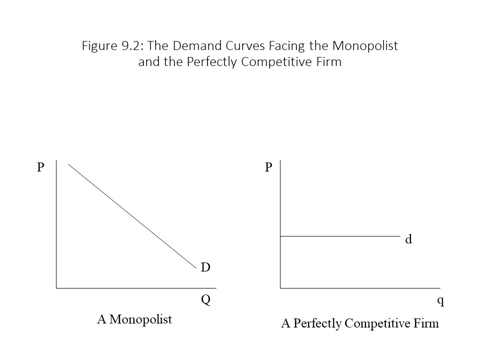
 Clearly, the firm’s TR in this case is $50 (= $5 per unit times 10 units) and is represented as the area of the rectangle in the graph. The average revenue (AR) can also be calculated as follows:
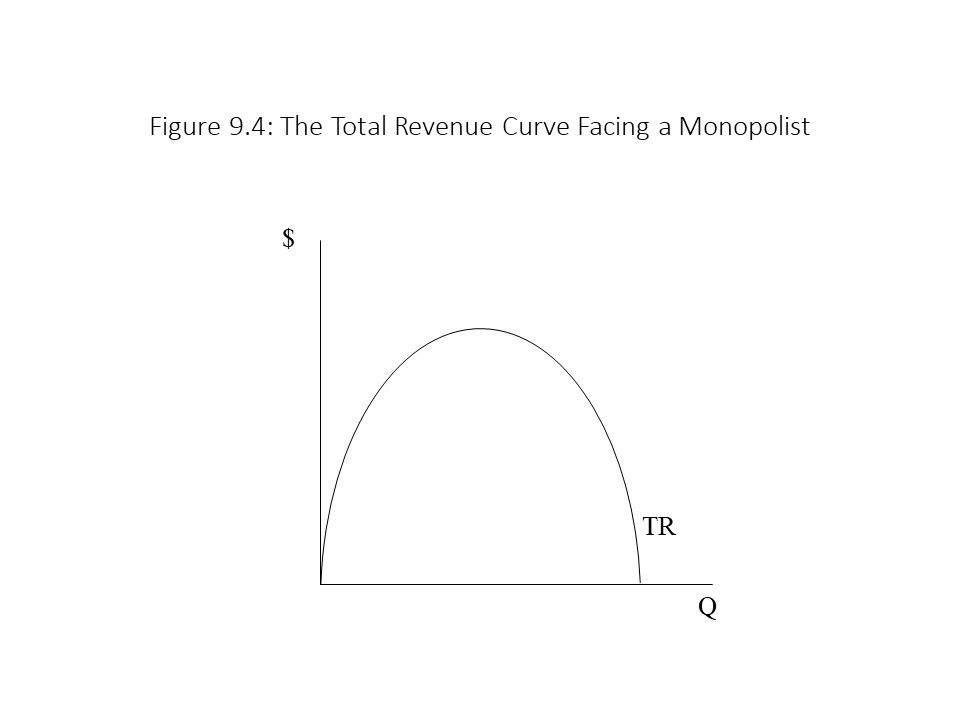 In Chapter 5, we learned that the reason for this shape is that at high prices demand is elastic and so price cuts lead to larger percentage increases in quantity demanded, which causes TR to rise overall. Once the price falls below the point of unit elasticity, demand becomes inelastic and further price cuts lead to smaller percentage increases in quantity demanded. As a result, TR falls. The pattern of TR as output changes is much more complicated for a monopolist than for a perfectly competitive firm. In the last chapter, we learned that a perfectly competitive firm’s TR rises continuously in a linear fashion because the firm faces a constant price as output rises. In the case of the monopolist, the firm is cutting price to sell additional units of output, and the changing demand elasticity causes TR to rise and then fall.
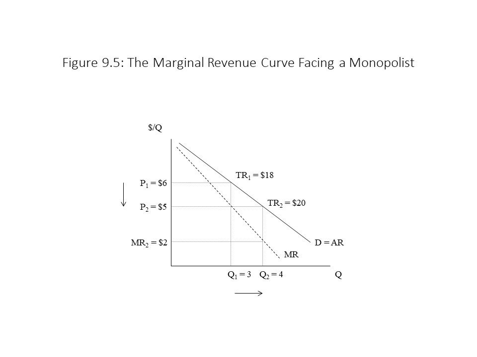 In Figure 9.5, the price falls from $6 per unit to $5 per unit, and the quantity demanded subsequently rises from 3 units to 4 units. The TR increases from $18 to $20 indicating that the firm is selling in the elastic portion of the market demand curve. The MR of the fourth unit of output may be calculated as follows:
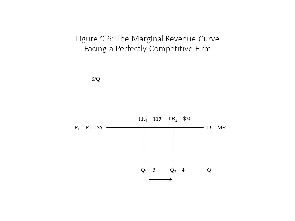 Using the information in Figure 9.6, we can see that the MR is calculated as follows:
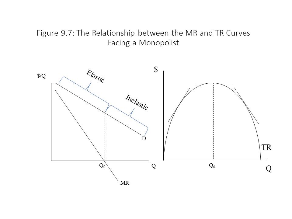 It should be clear that in the elastic portion of the demand curve, the MR is positive because the slope of the TR curve is positive. Similarly, at the peak of the TR curve where demand is unit elastic, the MR is equal to zero because the slope of the TR curve is zero. Finally, in the inelastic portion of the demand curve where the TR is falling, the MR must be negative because the slope of the TR curve is negative.
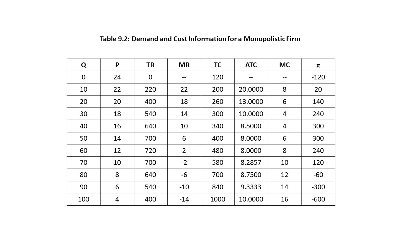
 It is important to notice that even though the profit-maximizing output level is found directly below the MR = MC intersection, the profit-maximizing price that is charged is found above the intersection on the market demand curve. The area of the shaded box represents the firm’s economic profit of $300, which may be calculated as the product of the amount by which P exceeds ATC (= $6 per unit) and the quantity sold (= 50 units). Alternatively, TR is $700 (= $14 per unit times 50 units) and TC is $400 (= $8 per unit times 50 units). The economic profit of $300 is simply the difference between the two amounts.
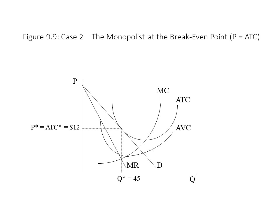 In Figure 9.9, the firm maximizes its economic profit by producing 45 units of output. This output level corresponds to the MR = MC intersection, and the price of $12 per unit at this output level is clearly above AVC. In fact, at Q = 45 units, the price equals the ATC. As a result, the firm’s TR is $540 (= $12 per unit times 45 units) and the firm’s TC is $540 (= $12 per unit times 45 units). Its economic profit is, therefore, equal to zero and so it is not represented as a shaded area in the graph. It should be recalled that this situation is acceptable to the monopolist because the firm is covering all its costs, including the opportunity cost of producing in this industry. Greater economic profits are always desired, of course.
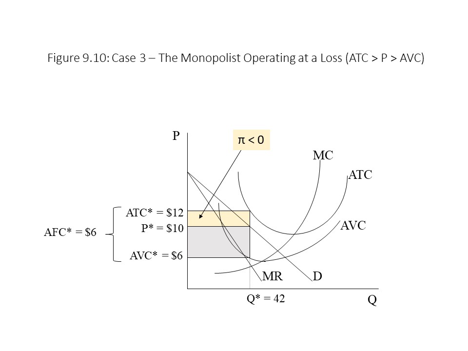 At that output level, MR = MC but also the profit-maximizing price of $10 is above the AVC of $6. The firm’s TR in this case is $420 (= $10 per unit times 42 units), and the firm’s TC is equal to $504 (= $12 per unit times 42 units). The economic profit then is equal to -$84 (= $420 – $504), which is also equal to the area of the top shaded box in Figure 9.10. If the firm is suffering a loss as indicated by its negative profit, then why does the firm operate in the short run? The reason is that the loss from shutting down would be even larger. As we discussed in Chapter 8, whenever a firm shuts down in the short run, its economic profit is equal to –TFC. The TFC can be calculated as the product of the AFC and the level of output. In this case, the TFC is equal to $252 (= $6 per unit times 42 units), which is also equal to the combined area of the two shaded regions in Figure 9.10. Clearly, an economic profit of -$252 is much worse for the firm than an economic profit of -$84. Therefore, the monopolist will choose to operate in the short run at a loss.
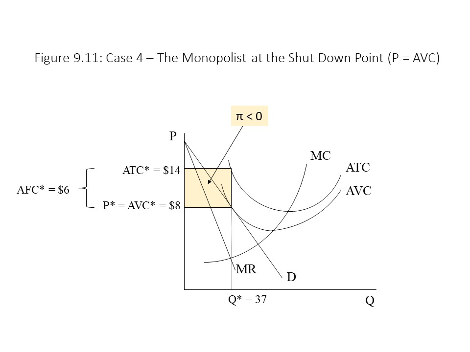 In this case, the firm charges a profit-maximizing price of $8 per unit, which is also equal to the firm’s AVC at this output level. Because the shutdown rule states that the firm will produce where MR = MC if P is greater than or equal to AVC, we conclude that the firm will operate in this case. The firm’s TR in this scenario is equal to $296 (= $8 per unit times 37 units). The firm’s TC is equal to $518 (= $14 per unit times 37 units). Therefore, the economic profit is equal to -$222. In addition, the firm’s TFC is equal to $222, which may be calculated as the product of AFC (= $6) and Q (= 37 units). Therefore, if the firm shuts down, it will suffer an economic loss of $222 (= -TFC), which is exactly equal to its loss from operating. In Figure 9.11, the shaded region represents both the TFC and the economic loss from operating. Even though the firm is indifferent between operating and shutting down, we conclude that the firm operates.
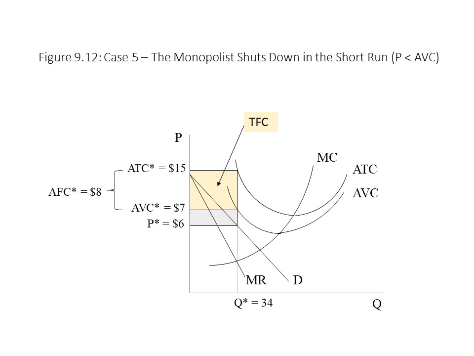 In this case, the firm produces no output because the price of $6 per unit, which is directly above the MR = MC intersection, is below the AVC of $7 per unit. Because the monopolist shuts down, its TR is $0 and its TVC is $0. It must still pay its TFC and so its economic profit is equal to –TFC. As always, the TFC may be calculated as the product of AFC and Q, which is here equal to $272 (= $8 per unit times 34 units). The firm’s economic loss of $272 is depicted as the top shaded box in Figure 9.12. If the firm were to produce 34 units and charge a price of $6 per unit, then its economic loss would be much greater. In that case, the monopolist’s TR would be $204 (= $6 per unit times 34 units), its TC would be $510 (= $15 per unit times 34 units), and its economic profit would be -$306 (= $204 – $510). The economic loss in that case would be equal to the combined area of the two shaded boxes in Figure 9.12. As a result, the firm opts to shut down and limit its losses to the TFC.
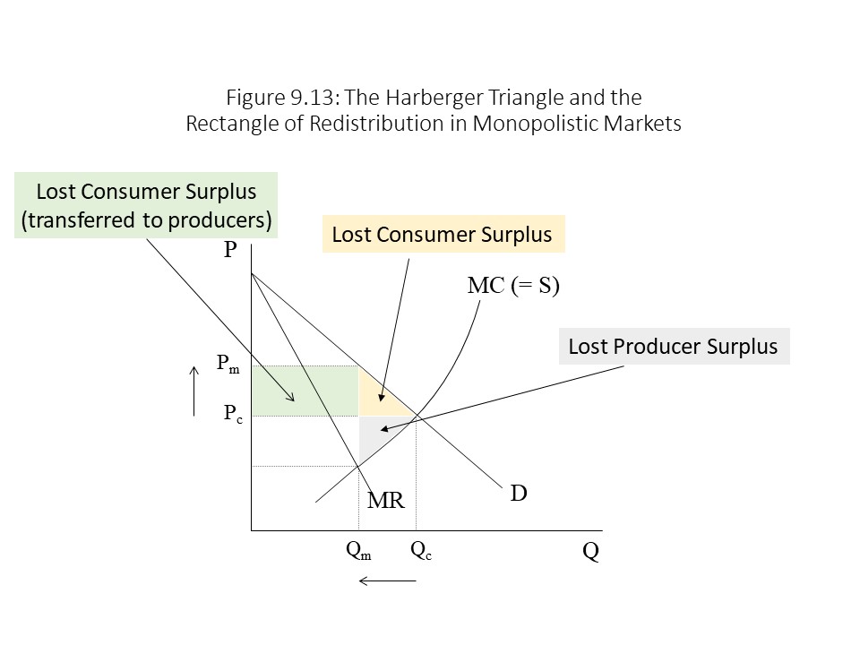 In Chapter 8, we learned that the marginal cost (MC) curve of a perfectly competitive firm is the same as the perfectly competitive firm’s supply curve (for MC above minimum AVC). It followed that the aggregation of the MC curves of all the perfectly competitive firms in the industry would yield the market supply curve. If we assume that the monopolist operates with the same production technology as the perfectly competitive firms, then we can assume that the monopolist’s MC curve is identical to the market supply curve that would emerge if the market was perfectly competitive. For this reason, the monopolist’s MC curve in Figure 9.13 is also labeled as a perfectly competitive market supply curve (= S). This approach allows us to compare the efficiency effects of the two market structures on the same graph.
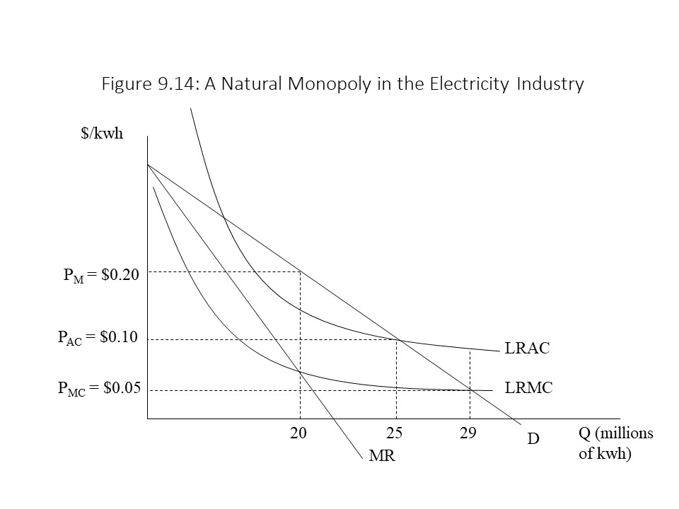 In Figure 9.14, the quantity of output is measured in millions of kilowatt hours (kwh) used per month. The price and unit costs are measured in dollars per kilowatt hour. Economies of scale are clearly present as can be seen from the declining LRMC and LRAC curves. The monopolist also faces a downward sloping demand curve and has a corresponding MR curve that declines more quickly than price. If the monopolist is allowed to operate freely, it will maximize its economic profit by selling 20 million kwh at a price of $0.20 per kwh. Because the monopoly price (PM) exceeds LRAC at 20 million kwh, clearly the monopolist will earn an economic profit.
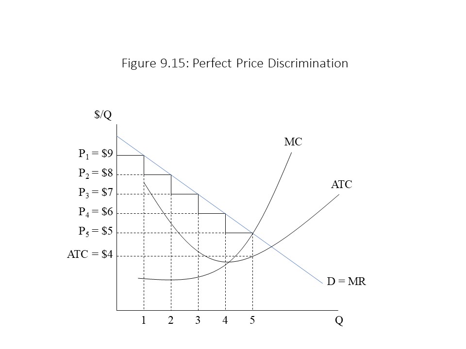 The major difference between this graph and the graph of the single pricing monopolist is that this monopolist’s MR curve is identical to the demand curve facing the firm. With a single pricing monopolist, the MR curve is steeper than the demand curve because the firm must cut the price on all units sold to sell another unit. When the monopolist can perfectly price discriminate, however, it does not need to cut the price on other units sold to sell one additional unit. As a result, the MR of an additional unit is the same as the price. Therefore, the market demand curve and the MR curve are the same in the case of perfect price discrimination. In Figure 9.15, the first unit is sold for $9 per unit, which is the maximum price that a consumer is willing and able to pay for that unit. The second unit sells for $8. Notice that the first unit still sells for $9 even though the second unit sells for $8 because perfect price discrimination occurs in this case. The MR of the second unit then is $8 because TR rises by the full amount of the price of that unit. The third, fourth, and fifth units sell for $7, $6, and $5, respectively. Notice that the monopolist will stop producing at 5 units because at this point MR = MC. The firm’s TR is calculated as the sum of the different prices charged as follows:
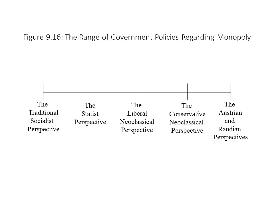 We will briefly discuss each of these responses beginning with the neoclassical perspectives since we have already explored the neoclassical theory of monopoly in detail. According to conservative neoclassical economists, the ideal market structure is the perfectly competitive one. Therefore, efficiency can be enhanced by breaking up monopolies into competing firms, effectively transforming a monopolistic market structure into a perfectly competitive market structure. The notion that government intervention can be used to create a more competitive environment is one that has a long history in the United States. The 1890 Sherman Act was the first major piece of federal legislation to outlaw unreasonable restraints of trade. In the early twentieth century, federal action was taken against Standard Oil, U.S. Steel, American Tobacco, and other firms because they had allegedly established illegal monopolies in their industries. The Clayton Act of 1914 and the creation of the Federal Trade Commission (FTC) that same year to enforce the nation’s antitrust laws further strengthened this instrument of federal control over markets. The conservative neoclassical perspective takes seriously the benefits of perfect competition, but its proponents prefer that this federal tool be used conservatively (i.e., only when a clear and convincing case can be made that a monopoly is firmly established in a specific industry and is harming consumers).