Construct two key measures of industry concentration
Identify the key characteristics of monopolistic competition in neoclassical theory
Explain how monopolistically competitive firms behave in the short run and long run
Describe the social consequences of monopolistic competition
Outline the key characteristics of oligopoly in neoclassical theory
Explore several neoclassical oligopoly models
Investigate the game theoretic concepts of dominant equilibrium and Nash equilibrium
Examine a Post-Keynesian markup pricing model
Two Measures of Industry Concentration
In this chapter we will explore imperfectly competitive markets. These market structures fall in between the neoclassical ideal of perfect competition and its antithesis of pure monopoly. The number of firms in an industry is a major determinant of a market’s location along the market power spectrum. Markets with many firms (other things equal) are more competitive and are considered to have less concentrated industries. Markets with fewer firms (other things equal) are less competitive and are considered to have more concentrated industries.
In chapter 8, it was pointed out that imperfectly competitive market structures include monopolistic competition and oligopoly (see Figure 8.2). Monopolistically competitive markets have relatively low degrees of industry concentration whereas oligopolistic markets have relatively high degrees of industry concentration. Because the market power spectrum is continuous, we require a measure of industry concentration that allows us to identify the degrees of market power in different markets relative to one another. In this section, we will introduce two different measures of industry concentration that many economists use to compare different markets.
Before we construct these measures, we must introduce a very important definition that will serve as the building block for our measures of industry concentration. A firm’s market share (Si) refers to the percentage of the market’s total sales revenue for which the ith largest firm is responsible during a given period. For example, in a specific industry, S2 refers to the second largest firm’s market share. Suppose that the second largest firm’s TR is $10,000 per month (TR2) and the total revenue earned in the entire market is $100,000 per month (TRM). In that case, S2 is defined and calculated for this case as follows:
In this case, the second largest firm has 10% of the market. It should be noted that the final calculation is 10 rather than 10%. That is, the 10% is implied. This point is important because the correct calculations of the measures that we construct require the omission of the percentages to obtain the correct answer as we shall soon see.
The first measure of industry concentration that we will introduce is referred to as the four-firm concentration ratio. Simply put, it is the combined market share of an industry’s four largest firms. It is defined as follows:
For example, suppose that an industry consists of the following market shares: 10, 20, 30, 25, and 15. Notice that these market shares sum to 100. Therefore, this industry contains exactly five firms. The four-firm concentration ratio in this case is 90 (= 30+25+20+15) because the smallest firm is excluded. This market appears to be highly concentrated because the four largest firms control 90% of the market.
The four-firm ratio appears to provide a sound measure of industry concentration. The larger it is, the more concentrated the industry is. The smaller it is, the less concentrated the industry is. A problem arises, however, when we consider examples of a specific sort. For example, consider two industries in which the market shares are 50 and 50 in Industry A and 25, 25, 25, and 25 in Industry B. In each case, the four-firm concentration ratio is 100. This result suggests that the two industries are equally concentrated. Our intuition, however, tells us that the industry with only two firms is significantly more concentrated than the industry with four firms. The four-firm ratio appears to be a deficient measure in the sense that it does not make distinctions between different industries that are as precise as we would prefer.
For this reason, we now introduce a second measure of industry concentration that is free from the defects of the four-firm ratio. The second measure of industry concentration is called the Herfindahl-Hirschman Index (HHI). It is named after the American economist Orris Herfindahl and the German economist Albert Hirschman. This measure is defined as follows for n firms in an industry:
The reader should notice two key differences between the four-firm ratio and the HHI. Unlike the four-firm ratio, the HHI includes every market share in the industry, not just the market shares of the largest four firms. Additionally, each market share is squared before the terms are added together. To understand why these changes have been made, let’s return to our example involving industries A and B from earlier. The HHI in Industy A (HHIA) and in Industry B (HHIB) are calculated as follows:
Whereas the four-firm ratio suggests that the two industries are equally concentrated, the HHI indicates that Industry A is twice as concentrated as Industry B. This result is much more consistent with our intuition and is an important reason to rely on the HHI, particularly when one is trying to make careful distinctions between levels of industry concentration. It should now be clear as well why the HHI includes the squaring of the market shares. The squaring technique allows the larger market shares to count much more heavily in the overall index than the smaller market shares. The inclusion of all market shares also allows us to obtain a more precise measure.
The HHI may also take on a much larger range of values than the four-firm ratio. That is:
In the extreme case in which a single firm has a market share of 100, the HHI equals 10,000 (= 1002). This case is the case of pure monopoly, and it should be noted that this situation is the only one that leads to a HHI of 10,000. The four-firm ratio, however, is 100 just like we found for Industries A and B. The lower extreme for the HHI is just above zero. Clearly, the only way to have a HHI of 0 is for all firms to have zero market shares, which means that the market simply does not exist. Therefore, for any existing markets, the smallest HHI is just above zero. Such a market would be very close to being perfectly competitive due to the huge number of very small firms. It is important not to focus on the specific value of the HHI. The index value by itself means rather little. What is important is the index value of one industry relative to another. The higher the index value is, the more concentrated is the industry.
The Antitrust Division of the United States Justice Department considers a HHI below 1,500 to be an unconcentrated industry, a HHI between 1,500 and 2,500 to be a moderate degree of concentration, and a HHI above 2,500 to be a high degree of concentration.[1]
Using data from the Economic Census provided by the United States Census Bureau,[2] we consider a few examples of unconcentrated industries shown below:
In 2002, the four-firm concentration ratio in animal food manufacturing was 39.3 and the HHI for the 50 largest firms was 636.6.[3]
The 2002 four-firm ratio in flour milling and malt manufacturing was 38.2 and the HHI for the 50 largest firms was 524.4.
The 2002 four-firm ratio in sugar manufacturing was 52.8 and the HHI for the 50 largest firms was 855.5.
A few examples of moderately concentrated industries are below:
In 2002, the four-firm concentration ratio in beet sugar manufacturing was 85.3 and the HHI for the 20 largest firms was 2,208.9.
The 2002 four-firm ratio in cookie and cracker manufacturing was 70.9 and the HHI for the 50 largest firms was 1,901.2.
The 2002 four-firm ratio in tortilla manufacturing was 59.3 and the HHI for the 50 largest firms was 2,355.4.
A few examples of highly concentrated industries are below:
In 2002, the four-firm concentration ratio in tobacco stemming and redrying was 84.2 and the HHI for the 20 largest firms was 2,905.9.
The 2002 four-firm ratio in house slipper manufacturing was 94.3 and the HHI for the 20 largest firms was 2,943.5.
The 2002 four-firm ratio in glass container manufacturing was 87.1 and the HHI for the 50 largest firms was 2,548.1.
Notice that tobacco stemming and redrying appears less concentrated than glass container manufacturing when we compare the four-firm ratios for the two industries, but tobacco stemming and redrying appears more concentrated than glass container manufacturing when we consider the HHI for the two industries. The two measures sometimes lead to contradictory results, but as we have seen, the HHI leads to more precise results than the four-firm ratio. Nevertheless, the four-firm ratio has a greater intuitive meaning and so it is often considered as well when investigating the degree of concentration in an industry. Now that we have a method of measuring industry concentration, we can explore the characteristics of the imperfectly competitive market structures that fall in between the extremes of perfect competition and pure monopoly.
Characteristics of Monopolistic Competition
Monopolistically competitive markets have three major features, two of which suggest a competitive market structure and one of which suggests a more monopolistic market structure. The two characteristics that contribute to the competitive nature of this market structure are the relatively large number of sellers and the absence of barriers to entry and exit in the long run. The characteristic that contributes to the monopolistic nature of this market structure is the tendency of all firms in the industry to produce products with slight differences that they promote aggressively through advertising. It is important to recognize that the differences need not be real or actual differences. If the consumer perceives a difference to exist across products in an industry, we may regard the market structure as monopolistically competitive. For example, doctors may tell patients that no significant differences exist across different types of aspirin, but the companies that produce aspirin promote their specific brands with great vigor. If consumers believe the differences exist, then each firm will possess some degree of market power. Other examples of monopolistically competitive markets include the markets for restaurant meals and auto repairs. Sometimes the factor that differentiates one product from another is nothing more than the location of the seller.
One good example of a monopolistically competitive market is the market for celebrity scents. As of 2009, firms were releasing at least 500 different kinds of celebrity perfume and cologne each year with department stores selling millions of bottles. Slight product differentiation is the source of each firm’s market power in this market. Firms have developed celebrity perfumes for Jennifer Lopez, Gwen Stefani, and Sarah Jessica Parker. Rapper 50 Cent also has a fragrance called Power by 50. Fans that waited at Macy’s in midtown Manhattan to buy a bottle of the new cologne had the good luck to have their photograph taken with the famous rapper. One fan exclaimed, “It’s him, it’s not the perfume. I can’t explain it, it’s like an energy you carry.”[4] Clearly, the uniqueness of the product often stems as much from the perceptions of the consumer as it does from the characteristics of the product itself.
Because each firm in a monopolistically competitive market has some market power, each firm faces a downward sloping demand curve for its specific product as shown in Figure 10.1.
Figure 10.1 also shows the graph of a downward sloping demand curve facing a pure monopolist. Two important differences between the two graphs should be noted. First, whereas the demand curve facing the pure monopolist is the entire market demand curve, the demand curve facing the monopolistically competitive firm is only a segment of the market demand. Second, the pure monopolist tends to face a much more inelastic demand curve because no close substitutes for the product exist. Therefore, consumers will be much less responsive to price changes when the market is purely monopolistic because they cannot find good substitute products. A monopolistically competitive firm faces competition from firms that produce close substitutes. The widespread availability of substitutes suggests that the demand curve facing the monopolistically competitive firm will be far more elastic since consumers can respond to price changes more easily.Figure 10.2 shows two possible short run scenarios for the monopolistically competitive firm.Depending on the relationship between the demand curve facing the firm and the unit cost curves, the firm may experience positive economic profits or negative economic profits in the short run. If the demand facing the firm is relatively high and unit costs are relatively low, then the firm will enjoy short run economic profits. If the demand facing the firm is relatively low and unit costs are relatively high, then the firm will suffer short run economic losses.Figure 10.3.
The reader should notice in Figure 10.3 that the demand curve facing the firm is just tangent to the ATC curve above the MR = MC intersection. At this point, price and ATC are the same and so economic profits are equal to zero in this case. How does this long run adjustment to zero economic profits occur? Two possible scenarios exist:
1. Economic profits exist in the short run, leading to the following:
Firms enter the industry in the long run.
The firms in the industry lose market share to the entering firms causing the individual demand curves that they face to shift leftward.
This adjustment continues until P = ATC and economic profits are equal to zero.
2. Economic losses exist in the short run, leading to the following:
Firms exit the industry in the long run.
The remaining firms in the industry gain market share causing the individual demand curves that they face to shift rightward.
This adjustment continues until P = ATC and economic profits are equal to zero.
The consequences of monopolistic competition are relatively straightforward. First, monopolistically competitive markets lead to inefficiency. Markup pricing exists (P > MC), which monopolistically competitive firms achieve by restricting their production levels below those that would prevail in a perfectly competitive market. Furthermore, least-cost production is not achieved because ATC exceeds the minimum ATC. In Figure 10.3, ATC* is higher than the minimum ATC that exists at the intersection between MC and ATC. The monopolistically competitive firm thus operates at less than optimal capacity. The conclusion that monopolistically competitive firms have a chronic problem of under-utilization of plant capacity is referred to as the excess capacity theorem of monopolistic competition.
Recall that the more unique the product is (i.e., the more differentiated it is), the steeper the demand curve will be because fewer close substitutes exist for the product. Similarly, if less product differentiation exists, then the demand curve is flatter because more close substitutes exist. In the extreme case that zero product differentiation exists, the market is once again perfectly competitive and the demand curve is perfectly horizontal. In that case, the MR = MC intersection will occur at the minimum point on the ATC curve. Hence, the problem of inefficiency in a monopolistically competitive market worsens as the products become increasingly differentiated. The increasing amount of differentiation gives individual firms more market power, which they use to restrict output further to raise prices and economic profits.
On the other hand, most consumers value some product differentiation. For example, if all firms in the shoe industry only produce one style of shoe, then the market will be perfectly competitive. A larger number of shoes would be produced at a lower per unit cost and price. Would our society suffer a different kind of loss, however, due to everyone wearing the same style of shoe? It would seem to be so. We would lose the ability to express our uniqueness in this way. Most of us would be willing to pay something extra for that opportunity of self-expression. How much more we are willing to pay for product variety is the question that is highly debatable. Our answers will surely vary depending on the specific good in question. A tradeoff thus exists between product variety and economic efficiency.
Characteristics of Oligopoly
Oligopolistic markets have several defining characteristics. These are markets dominated by a few large firms. Oligopolistic markets may have just two or three firms or even nine or ten firms. The specific number of firms is not rigidly defined. Again, the degree of concentration in an industry is measured along a continuum. For decades, the U.S. automobile market was dominated by the “Big Three” (i.e., General Motors, Ford, and Chrysler). In the beer industry, the “Big Five” in the early 1990s included Anheuser Busch, Miller, Stroh, Coors, and Heilemann. Oligopolies have also existed in the markets for breakfast cereal, steel, and military weaponry.
Also required for a market to be oligopolistic is that each firm has considerable market power, which is the result of barriers to entry that discourage competition. Such entry barriers might include patents, or large startup costs that generate economies of scale. The final characteristic of oligopoly markets is that the firms in the industry behave strategically when setting prices and output levels. That is, each firm sets its price while considering the prices and likely reactions of its competitors. This characteristic sharply distinguishes this market structure from the other market structures. In a perfectly competitive market structure, each firm takes the price as given and ignores the actions of competitors. In a purely monopolistic market, no competitors exist. In a monopolistically competitive market, firms might strive to differentiate their products, but at a point in time, the prices they charge are entirely determined by the demand segments they face and the production costs they incur.
The element of strategic interaction makes it very difficult to model oligopoly behavior. As a result, no single oligopoly model is dominant within neoclassical economics. We will consider several models as well as explore how a special subfield of economics called game theory may shed light on the behavior of oligopolistic firms.
A Simple Duopoly Model
Sometimes oligopoly markets only contain two firms. These special cases of oligopoly markets are called duopoly markets. Suppose that you and your competitor are the only two sellers in the market for baseball cards. Your supply curve and your competitor’s supply curve are shown in Figure 10.4.[5]
The supply price refers to the minimum price that these sellers are willing and able to charge for the corresponding output level. Initially, your supply price and your competitor’s supply price are P1 = $2.00 per baseball card and your output levels are each q1. Now assume that you and your competitor think strategically about each other’s price. Let’s assume that pricing takes place in a series of rounds with each seller reacting to the other seller’s price every other round. Further suppose that you and your competitor each decide that you will always cut the price per card by $0.50 below the price set by the competition. Finally, assume that your competitor is the first to act. Your competitor cuts the price to P2 = $1.50, undercutting you by $0.50. Since you follow a similar strategy, you decide to cut your price to P3 = $1.00, thus cutting your price in half and undercutting your competitor by $0.50. In response, your competitor cuts price to undercut your new price and so sets a price of P4 = $0.50. Your stubborn adherence to this cutthroat strategy leads you to reduce your price to zero and your competitor follows. If the two sellers adhere strictly to these pricing rules, a zero price/zero quantity equilibrium is the result since quantities supplied decline with the price cuts.
The problem with this model, of course, is that actual oligopoly markets do manage to persist without price wars completely undermining production. For one thing, firms have production costs and so they may not be willing to cut prices so low that they suffer extensive losses. Also, firms are able to grab a larger market share when they undercut competitors and that factor is not taken into account in Figure 10.4. Therefore, we seem to require models that can explain how oligopoly firms may coexist while accounting for the actions of their competitors and earning positive economic profits. It is to these models that we now turn.
The Kinked Demand Model of Non-Collusive Oligopoly
In 1939, the Marxian economist Paul Sweezy introduced what has become known as the kinked demand curve model of non-collusive oligopoly.[6] It is rare that a Marxian economist develops a model that becomes widely taught by neoclassical economists. The kinked demand curve model is an important example of how sometimes ideas developed within one school of economic thought spill over into other schools of economic thought. Certainly, not all neoclassical economists accept the validity of this model’s conclusions, but it has been incorporated into most mainstream economics textbooks.
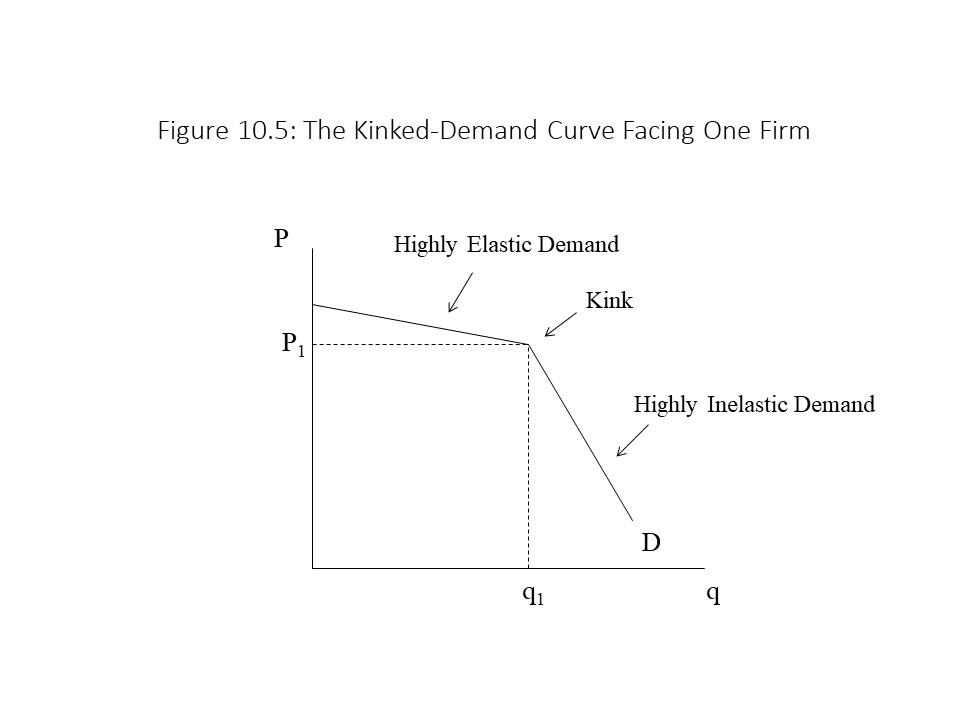
The purpose of the model is to explain how oligopoly firms manage to establish stable prices in the marketplace without relying on collusion. That is, price wars are somehow avoided in these markets even though the firms never coordinate with one another to explicitly fix prices. Because the purpose is to explain the rigidity or “stickiness” of the price rather than the level of the price itself, the model assumes that one of the oligopolistic firms is already charging a specific price P1 and producing a specific quantity q1 as shown in Figure 10.5.
Given the original price of P1, we need to determine the shape of the demand curve facing this firm. To derive the demand curve facing the firm, we ask what will happen if this firm raises its price above P1. Because we are assuming that firms think strategically, it is reasonable to expect that when this firm raises its price, the other firms will not follow with a price increase. By not following with a price increase, they can capture a larger share of the market. As a result, when this firm raises its price, its customers will react by purchasing the product from the firm’s competitors. That is, consumers will be very responsive to the price increase and the quantity demanded will fall significantly. In other words, the demand curve facing the firm is very elastic above the price of P1.
On the other hand, suppose this firm reduces its price below P1. Because we are assuming that firms think strategically, it is reasonable to expect that when this firm cuts its price, the other firms will follow with a price cut. By following with a price cut, the other firms can prevent this firm from capturing a larger share of the market at their expense. As a result, when this firm cuts its price, it will not be able to expand its sales much at all. That is, consumers will be very unresponsive to the price cut and the quantity demanded will only increase a small amount due to new customers entering the market. In other words, the demand curve facing the firm is very inelastic below the price of P1.
Because the demand curve is relatively flat above P1 and relatively steep below P1, the demand curve facing the firm has a kink at a price of P1. The next step is to determine the firm’s marginal revenue (MR) curve. We have seen that a downward sloping demand curve has a corresponding MR curve that declines more quickly than demand. Again, the reason is that when the firm cuts the price to sell another unit, it must cut the price of all units sold. As a result, the revenue rises by less than the price of the additional unit. In the case of a kinked demand curve, we essentially observe two downward sloping demand curves joined at the kink. Each section then should have a downward sloping MR curve that corresponds to it. Figure 10.6 shows the MR curve for an oligopolistic firm facing a kinked demand curve.
In Figure 10.6, the MR curve has a gap in it. The gap occurs at the same output level of q1 at which the kink occurs. This gap in the MR curve can be explained intuitively. Imagine that the firm is cutting the price at levels above P1. The MR is given by the flatter portion of the MR curve. Once the firm reaches P1, a substantial price cut is needed to sell one more unit. This large price cut causes the price to drop considerably for all other units sold and so the MR plummets, creating a gap in the MR curve. If the firm then continues to cut price along the inelastic portion of the demand curve, the MR falls steadily along the steeper portion of the MR curve.Figure 10.6. The MC curve of the oligopolistic firm is determined by the very same factor discussed previously: production technology. That is, the MC declines due to specialization and division of labor and then rises due to diminishing returns to labor. We can now determine the profit-maximizing output and price. Following the rule that the firm will equate MR and MC, if the firm’s MC is MC1 then the firm will produce where MR and MC1 intersect. Technically, a discontinuity occurs in the MR curve and so no intersection occurs. Despite this technicality, the firm will increase its profit by producing more when MR exceeds MC, and the firm will increase its profit by producing less when MC exceeds MR. This tendency leads the firm to produce at an output level of q1. The price charged is then set up on the demand curve above this output level at P1. Interestingly, we obtain the same result if marginal cost declines to MC2. That is, the firm will set price and output at the kink in the demand curve. The implication is that unit cost can fluctuate significantly with no effect on price or output. That is, the model provides an explanation for price rigidity in oligopolistic markets. Even if unit cost drops significantly, firms will hesitate to cut price because doing so will cause a price war. Similarly, even if unit cost rises significantly, firms will hesitate to raise price because doing so will cause a loss of market share. Price changes, therefore, lead to a reduction in the firm’s economic profits. If all firms reason in a similar manner, then price stability arises even without collusion.
It should be noted that price changes are possible in the kinked demand model. A rise in price might occur, for example, if MC rises a great deal. A rise in MC to MC3 will lead to a reduction in output below q1 and a rise in price above P1. A drop in MC to MC4 will lead to an increase in output above q1 and a decrease in price below P1. The point is not that prices never change in oligopolistic markets but only that they are less likely to change than in other market structures when production costs change. If you think about Coke and Pepsi, for example, these two firms do not collude. If they fixed prices, it would be illegal. Still, relatively stable and similar prices emerge in the market for soda. The author encountered another interesting case a few years ago at Wendy’s. A tomato shortage had caused the price of tomatoes to rise significantly. As a result, Wendy’s asked each customer who ordered a hamburger whether they would be willing to forego the slice of tomato that typically is included on a Wendy’s hamburger. In this case, the firm’s MC rose, and it made a special effort to enlist the help of customers in keeping MC down, all to avoid a price increase that might cost it market share if its competitors refused to follow the price increase.
The kinked demand curve model of oligopoly is useful for thinking about how stable prices may emerge in oligopolistic markets. It is subject to the criticism, however, that it only explains the stability of the product price and not its magnitude. For that reason, neoclassical economists have several other ways of thinking about oligopolistic behavior.
Two Additional Models: Collusive Oligopoly and Price Leadership
The kinked demand model of non-collusive oligopoly assumes that the firms do not explicitly agree on price. Each firm chooses its price and output independently even though each carefully considers what its competitors are doing and will do in response to a price change. If firms do collude, then essentially the firms will act as a pure monopoly. Such a collusive oligopoly is referred to as a cartel. Quite simply, a cartel is a group of firms that behaves as a single firm with respect to certain decisions, which might include the product price, the output level, or the market share for each cartel member. The most famous example of a cartel is probably the Organization of Petroleum Exporting Countries or OPEC. This international oil cartel, made up primarily of Middle Eastern oil producers, has manipulated oil prices at different times since it was first formed in the 1960s.
The major difference between a cartel and a purely monopolistic firm is that a cartel is much less likely to remain intact over time for several reasons.[7] First, cartel members are often located in different geographic regions. As a result, the individual demands that they face and the production costs they incur may be significantly different. As a result, it will be difficult for the firms to agree on an appropriate product price. Second, cartel agreements tend to be weaker when a larger number of firms belong to the cartel. That is, it is easier to reach and maintain a pricing agreement among three firms than it is among eight firms. Third, the temptation to cheat on the pricing arrangement is immense because a firm can capture a greater market share by secretly undercutting the other cartel members. When all firms begin to cheat, the cartel falls apart. Such temptations are greatest during periods of economic recession when falling demand leads to desperate attempts to attract new customers. Fourth, cartels are often slow to form because the firms in the market fear that a high cartel price will attract new competition in the market. Finally, the antitrust laws discussed in the last chapter serve as a major barrier to cartel formation in the United States. Firms accused of price fixing face federal prosecution, steep fines, and even criminal punishment for their efforts to rig markets in their favor.
In other markets, market-sharing agreements may emerge in which one large firm acts as the price leader and many small competitors follow along by setting the same price as the leader. The price leader ends up sharing the market with many small firms by means of an implicit agreement. For example, U.S. Steel acted as the price leader in the steel industry during the early twentieth century. U.S. Steel would publish price catalogs periodically in which it would announce its new prices. Smaller steel companies would inevitably follow along. When the steel companies deviated from this policy during the panic of 1907, U.S. Steel retaliated with even steeper price cuts that severely punished the smaller steel companies. With this implicit threat in place, the steel companies quickly learned that they must continue to follow the lead of U.S. Steel in the pricing of steel products. In the U.S. automobile industry in the mid-twentieth century, a similar pattern arose with General Motors serving as the price leader. The president of GM would announce new automobile prices in a speech and the other automakers would fall into line with similar prices.
Neoclassical economists use a price leadership model to investigate how the established price, market demand, and the cost structures of the different firms collectively determine how the market is divided between the price leader and the smaller competitors. Figure 10.7 provides a graph that represents the price leadership model for (let’s say) the automobile market.[8]
This graph is a bit involved and so we will discuss each piece before bringing all of them together to provide an explanation of how the market is divided when a price leader exists. First consider the market demand for automobiles (Dm). It is a downward sloping curve consistent with the law of demand. The small firms’ supply curve, on the other hand, is upward sloping consistent with the law of supply. As the price increases, the quantity supplied of the small firms rises because the higher price covers the higher marginal cost of production. If no other firms exist in this market, then the market will be perfectly competitive and the equilibrium price will be the competitive price of P2 where the supply of the small firms and market demand intersect.
Another firm does exist in this market, however, and it is the price leader. We wish to know what the demand curve is that faces the price leader in this market. We can derive the demand curve facing the price leader (DL) by asking how much of the market demand remains at each price after the small firms have selected their quantity supplied. For example, at a price of P2 the small firms produce enough to satisfy the entire market demand. Nothing remains then for the price leader and so the quantity demanded of the price leader’s product is zero at a price of P2. This point is one point on the demand curve facing the price leader. On the other hand, at a price of P1, the small firms produce nothing. The quantity demanded facing the price leader in that case is the entire quantity demanded in the market. This point is a second point on the demand curve facing the price leader. As the price declines from P2 to P1, the small firms’ quantity supplied falls continuously causing the price leader to acquire an increasing amount of the market demand until the price leader captures the entire market. The demand curve facing the price leader is, therefore, a downward sloping demand curve connecting the two points just mentioned.
Once we have determined the demand curve facing the price leader, it is a short step to obtain the MR curve for the price leader (MRL). It is also downward sloping and falls more quickly than the demand curve for the very same reasons provided previously whenever we have derived the MR curve from a downward sloping demand curve. Additionally, the MC curve for the price leader (MCL) is upward sloping due to the rising marginal cost of production, which stems from diminishing returns to labor.
We now have all the component parts, which we can bring together to complete the price leadership model. The price leader considers the situation and aims to maximize its economic profit. It sets MRL equal to MCL, as any profit-maximizing firm does, and produces QL*. To sell this amount of output, it must set the price up on the demand curve facing the price leader at P*. If the price leader sets the price up on the market demand curve then the price leader will not be able to sell QL* and the firm’s economic profit will not be maximized. The small firms follow the price leader and set the same price of P*. The quantity supplied of the small firms shows up in two different ways in this graph. At a price of P*, we can look at the small firms’ supply curve to see that the small firms will supply QS* at that price. Equivalently, the small firms produce enough to satisfy the market demand that remains after the price leader has set its output. Because QT* is the quantity demanded in the entire market at a price of P*, QS* must also equal the difference between QT* and QL*. That is, the small firms produce what is left over of the market demand after the price leader has taken its share of the market. We can express this result symbolically as follows:
The market is thus divided between the price leader and the small firms. Clearly, the price leader could capture the entire market by setting the price all the way down at P1. The price leader has no incentive to do so, however, because it would produce far more output than is profit-maximizing. If the firm produced at that output level, MC would far exceed MR. Contrary to what one might expect, it is profit-maximizing for the price leader to share the market with the smaller firms.
In general, oligopoly markets tend to be inefficient. In the kinked demand model, the cartel model (i.e., the pure monopoly model), and the price leadership model, the firms set price above MC. All such firms restrict output to maximize their economic profits. On the other hand, the large economic profits of oligopolistic firms enable them to invest in new production technologies that can enhance efficiency. Whether and to what extent these investments offset or cancel out the inefficiencies of oligopolistic firms is a question that may vary by industry.[9]
A Detour into Game Theory
Neoclassical economists also use an analytical method referred to as game theory to investigate the competitive interaction of oligopolistic firms. Game theory has been applied to many other topics in economics as well as other fields, including biology and political science. It is an analytical method that makes possible the study of strategic interaction between individual agents or players. In this section, we will discuss simultaneous games, in which all players simultaneously choose their strategies or courses of action.
The first game that we will consider has only two players: Player A and Player B. Each player has two possible strategies from which to choose. That is, a player may set a high price or a low price. Figure 10.8 shows a payoff matrix with four possible outcomes.
If both players set a high price, then outcome A is the result. If both players set a low price, then outcome D is the result. If player A sets a high price and player B sets a low price, then outcome B is the result. Finally, if player A sets a low price and player B sets a high price, then outcome C is the result. Each outcome has a set of payoffs associated with it, which may be interpreted as the economic profits that each player receives if that outcome occurs. If the payoff is negative, then it may be interpreted as an economic loss.
Our purpose is to determine which of the four outcomes will occur when the players simultaneously choose their strategies. The reader may be tempted to select outcome A because both players receive the highest payoffs when this outcome occurs. Although in this case outcome A is the correct outcome, this approach frequently does not lead to the correct outcome. The following approach may be used to arrive at the correct outcome:
If Player A sets a high price, then Player B sets a high price (since 200 > 75).
If Player A sets a low price, then Player B sets a high price (since 75 > -100).
In this case, we say that a high price is a dominant strategy for Player B, meaning that the best response of Player B is always to select the same strategy regardless of what Player A chooses to do. We now investigate Player A’s best responses to Player B’s possible strategies.
If Player B sets a high price, then Player A sets a high price (since 200 > -100).
If Player B sets a low price, then Player A sets a high price (since -50 > -100).
In this case, Player A also has a dominant strategy, which is to always set a high price. Both players, therefore, have dominant strategies. Because both players will choose to set a high price, the outcome of the game is outcome A, and each player receives a payoff of 200. When the equilibrium outcome of the game results from both players having dominant strategies, the outcome is called a dominant equilibrium. Outcome A is, therefore, a dominant equilibrium.
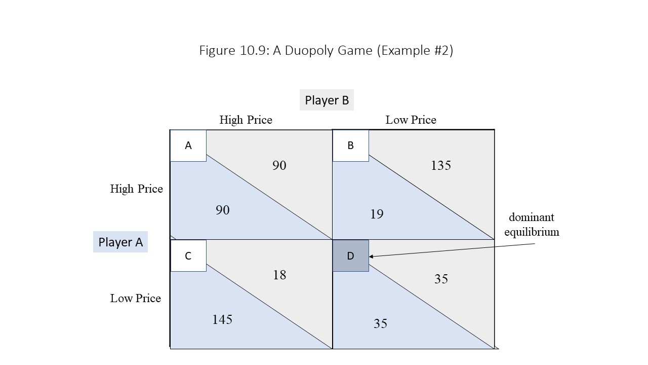
Consider the second game represented in Figure 10.9.
We will follow the same procedure that we used with the first game to determine the outcome of the game.
If Player A sets a high price, then Player B sets a low price (since 135 > 90).
If Player A sets a low price, then Player B sets a low price (since 35 > 18).
In this case, Player B has a dominant strategy to always set a low price regardless of the strategy that Player A chooses. Furthermore:
If Player B sets a high price, then Player A sets a low price (since 145 > 90).
If Player B sets a low price, then Player A sets a low price (since 35 > 19).
In this case, Player A also has a dominant strategy to always set a low price regardless of the strategy that Player B chooses. Since both players opt to set a low price, the outcome of the game is outcome D, and each player receives a payoff of 35. Because both players have dominant strategies, the outcome of the game is a dominant equilibrium.
The outcome of this game is especially interesting because each player receives a lower payoff than he or she would have received had both players set high prices. Essentially, what happens here is that a price war leads to a suboptimal outcome for both players. The reader might conclude that collusion would prevent this problem from arising. If each player agrees to charge a high price, then outcome A can be achieved. Is it true? Suppose the two players agree to charge a high price. Each player knows that its best response to the other player charging a high price is to charge a low price. Player A, for example, will enjoy a payoff of 145 rather than 90 by undercutting Player B. Similarly, Player B will enjoy a payoff of 135 rather than 90 when undercutting Player A. In other words, both players have an incentive to cheat on their pricing agreement. Since both players aim to maximize their payoffs, the pricing agreement falls apart. Game theory thus sheds light on the reason that cartel agreements are difficult to maintain except for short periods. The incentive to cheat is simply too great.
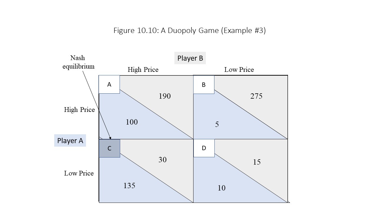
Consider a third game represented in Figure 10.10.
Again, we will follow our method of determining the outcome of the game.
If Player A sets a high price, then Player B sets a low price (since 275 > 190).
If Player A sets a low price, then Player B sets a high price (since 30 > 15).
We see here that Player B does not have a dominant strategy since Player B’s best response depends upon Player’s A’s choice of strategy. Furthermore:
If Player B sets a high price, then Player A sets a low price (since 135 > 100).
If Player B sets a low price, then Player A sets a low price (since 10 > 5).
Player A clearly has a dominant strategy to always set a low price regardless of which strategy Player B chooses. Still, in this case, the outcome is not immediately obvious since Player B does not have a dominant strategy. Nevertheless, we can arrive at the outcome if we assume that each player is able to anticipate the decision-making process of the other player. For example, if Player B can see that Player A will always set a low price no matter what Player B chooses, then Player B will choose her best response to Player A setting a low price. In this case, Player B will set a high price because setting a high price is Player B’s best response to Player A setting a low price. Outcome C is the result of this game.
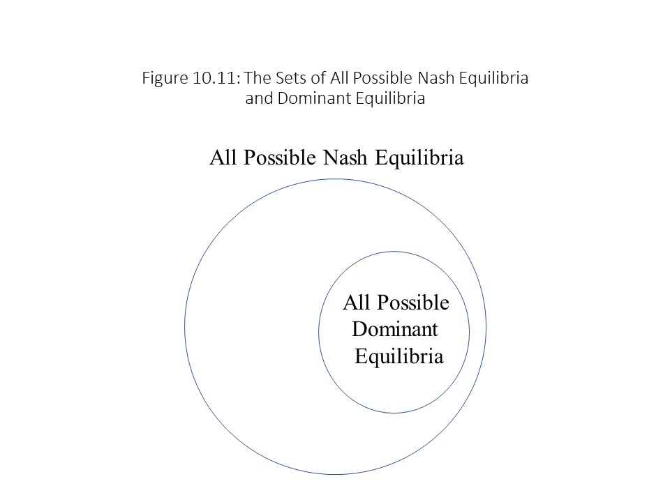
Because an outcome is called a dominant equilibrium only when both players have dominant strategies, outcome C is not a dominant equilibrium. Nevertheless, the outcome is a Nash equilibrium, which is a concept named after John Nash for his discovery of it in the 1950s and for which he was awarded the Nobel Prize in Economics in 1994. A Nash equilibrium exists when every player has chosen her best response given the strategies of the other players. Outcome C (A low and B High) is a Nash equilibrium because Player A’s best response is to always set a low price. Similarly, Player B’s best response to Player A’s low price is a high price. Clearly, not every Nash equilibrium is a dominant equilibrium as this example shows, but is every dominant equilibrium a Nash equilibrium? The answer is yes. A dominant equilibrium exists whenever both players have selected their dominant strategies and these strategies are always their best responses to whatever the other players have chosen. Figure 10.11 shows the relationship between the set of all possible Nash equilibria and the set of all possible dominant equilibria.
As the Venn diagram shows, every dominant equilibrium is a Nash equilibrium but not every Nash equilibrium is a dominant equilibrium.Figure 10.12.
Again, we will follow our method to determine the outcome of the game.
If Player A sets a high price, then Player B sets a high price (since 100 > 0).
If Player A sets a low price, then Player B sets a low price (since 200 > 0).
In this case, Player B does not have a dominant strategy. Furthermore:
If Player B sets a high price, then Player A sets a high price (since 200 > 0).
If Player B sets a low price, then Player A sets a low price (since 100 > 0).
Player A also lacks a dominant strategy. It will not be possible to determine the outcome of the game as we did in the third game because neither player can be sure what the other player will do. Nevertheless, it is possible to identify two Nash equilibria in this game. Notice that if Player A sets a high price, then Player B’s best response is to set a high price. Similarly, if Player B sets a high price, then Player A’s best response is to also set a high price. Therefore, when each player sets a high price, each player has chosen her best response to the other player. Outcome A is thus a Nash equilibrium. It should also be noticed that if Player A sets a low price, then Player B’s best response is to set a low price. Similarly, if Player B sets a low price, then Player A’s best response is to set a low price. When each player sets a low price then, each player has chosen her best response. Outcome D is thus also a Nash equilibrium. This game, therefore, has two Nash equilibria. Outcomes B and C are not Nash equilibria because neither player chooses her best response for those outcomes. Games with multiple Nash equilibria are thus possible.
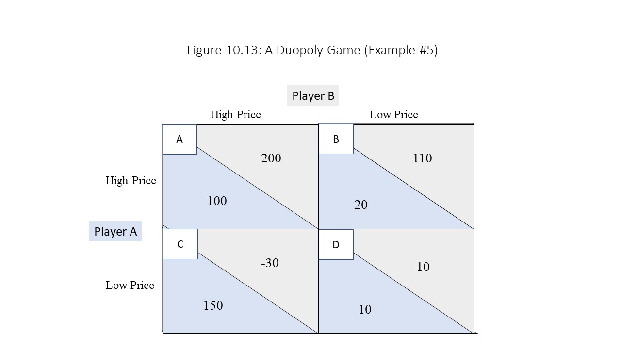
The final game we will consider also has a surprising outcome. Consider the fifth game represented in Figure 10.13.
Again, we will follow our method to determine the outcome of the game.
If Player A sets a high price, then Player B sets a high price (since 200 > 110).
If Player A sets a low price, then Player B sets a low price (since 10 > -30).
In this case, Player B does not have a dominant strategy since her best response depends upon Player A’s choice of strategy. Furthermore:
If Player B sets a high price, then Player A sets a low price (since 150 > 100).
If Player B sets a low price, then Player A sets a high price (since 20 > 10).
Again, neither player has a dominant strategy. Therefore, the outcome cannot be determined as in the third game. Can we identify any Nash equilibria though? Let’s see. If Player A sets a high price, then Player B will set a high price, but if Player B sets a high price, then Player A sets a low price. When considering this analysis of Figure 10.13, we fail to find the agreement we found when looking at the fourth game. Similarly, if Player A sets a low price, then Player B sets a low price, but if Player B sets a low price, then Player A sets a high price. Again, considering this analysis of Figure 10.13, we fail to find the agreement we found in the fourth game. Hence, no Nash equilibrium exists in this game. An alternative method of verifying that no Nash equilibrium exists is to consider each of the four outcomes in the game. For each outcome, we should ask whether each player has chosen her best response to the other player. If we answer in the negative for either player, then that outcome cannot be a Nash equilibrium. As the reader can see, these games have many possible outcomes!
A Post-Keynesian Markup Pricing Model
Post-Keynesian economists have a different model of oligopolistic behavior than the neoclassical models that we have explored in this chapter. As explained in Chapter 1, post-Keynesian economics is a complex body of thought that derives mostly from the ideas of John Maynard Keynes but which also contains elements of classical political economy, Marxian economics, Sraffian economics, and neoclassical economics. In this chapter, we will explore the post-Keynesian theory of pricing in oligopolistic markets in such a way that we see how some of these elements are brought together to provide a unique explanation of firm behavior.
Post-Keynesian economists distinguish between two types of markets that they refer to as “flexprice” markets and “fixprice” markets.[10] The flexprice markets are intensely competitive and prices are determined according to the laws of supply and demand.[11] The fixprice markets, on the other hand, are oligopolistic and have prices determined as the sum of the “normal cost of production” and a markup for profit.[12] Whereas flexprice markets tend to include markets for agricultural commodities and raw materials, fixprice markets include markets for finished, manufactured commodities.[13] For post-Keynesian theorists, the latter type of market is the most important in terms of understanding modern capitalist economies.[14]
The key issue in fixprice markets is the determination of the profit markup.[15] Post-Keynesian economists argue that the profit markup is established according to firms’ need for internal financing of new investment projects out of current profits.[16] Their aim is to maximize sales revenue or market share rather than short run profit.[17] That is, if firms anticipate greater future demand for their products, then they will increase the profit markup. The larger markup will generate larger profits which can be used to expand production plant capacity. Similarly, firms will reduce the profit markup if they anticipate a reduction in future demand for their products. The reduction will allow them to reduce the level of investment and avoid creating unnecessary additional plant capacity.[18] The change in the markup will cause the price to change in these markets. The only other factor that can cause the price to change in these markets is a change in the normal level of production cost.[19] Why then are these markets referred to as fixprice markets? Because short run changes in current demand do not affect the product price. Instead, firms will expand production (or output) to meet short run surges in demand and will reduce output in response to short run drops in demand. Firms are assumed to possess some excess production capacity that allows them to make these short run adjustments. In flexprice markets, on the other hand, short run changes in demand do affect product prices, as explained in Chapter 3 in the context of the neoclassical supply and demand model.
It is possible to represent the post-Keynesian theory of oligopolistic pricing more precisely. Let’s assume that the price is determined as the sum of short run unit cost (ATC) and the per unit profit markup as shown below:
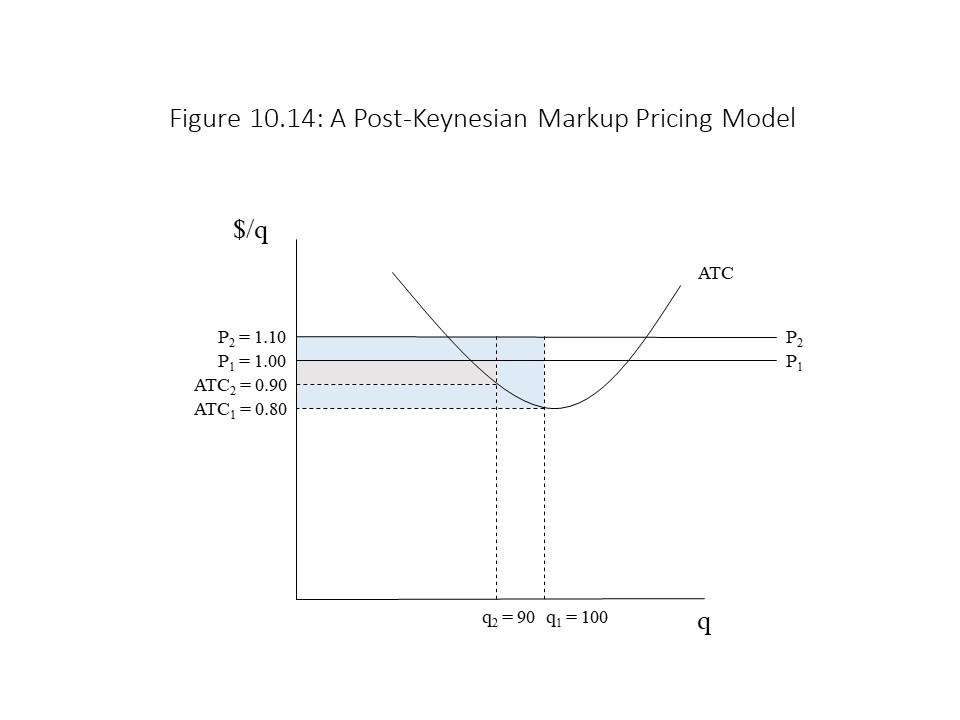
In this case, the ATC may be interpreted as the normal cost of production in the short run.[20] Figure 10.14 depicts the post-Keynesian markup pricing model.
Suppose the firm initially charges a price of $1.00 per unit and produces an output of 100 units. The ATC is $0.80 per unit in this case. The markup is $0.20 per unit. Notice that the firm has a small degree of excess capacity because it has not quite reached the lowest point on its ATC curve. The firm’s total profit in this case is $20 (= $0.20 per unit times 100 units). If a short run reduction in demand occurs, then the firm will maintain the price of $1.00 per unit but will reduce output from 100 units to 90 units. The firm keeps the price the same because this market is a fixprice market and short run changes in demand do not affect price. Post-Keynesian economists explain the reluctance to change price as stemming from firms’ fear that they might “spoil the market by damaging customer goodwill.” [21] The firm experiences an increase in excess plant capacity because it has reduced its output. Due to the failure to fully utilize its plant capacity and the gains from specialization, the per unit cost increases to $0.90 per unit. The markup thus falls to $0.10 per unit and profits decline to $9.00 (= $0.10 per unit times 90 units).
Suppose next that the firm expects an increase in the future demand for its product. The managers believe that plant capacity must be increased to meet the larger future demand. As a result, the firm increases its profit markup from $0.10 per unit to $0.20 per unit. This change will allow the firm to earn enough additional profit to finance the plant expansion using internal funds. The firm thus increases its price to $1.10. The firm’s profits now increase to $18 (= $0.20 per unit times 90 units). If a short run increase in demand restores current demand to its previous level, now the firm’s profits increase to $30 (= $0.30 per unit times 100 units). The firm is now charging a price of $1.10 per unit and incurring unit costs of only $0.80 per unit, generating a per unit profit of $0.30 per unit on these 100 units.
This analysis shows how oligopolistic firms may alter their production levels in the short run while maintaining constant prices in the face of changing current demand. At the same time, it shows how prices may be changed to support investment projects that will help satisfy higher expected future demand. The analysis also shows how profits vary at a microeconomic level as current demand rises and falls. This pattern of rising and falling profits with changing demand conditions is perfectly consistent with the post-Keynesian analysis of the business cycle that we will discuss in Chapter 14. The consistency of post-Keynesian microeconomic analysis and macroeconomic analysis is a point in its favor given how much difficulty neoclassical economists have faced with their efforts to create a synthesis of microeconomic and macroeconomic theory.
The model also shows how post-Keynesian economics is a blend of different bodies of thought. The belief that markets often fail to clear automatically is a central feature of Keynes’s perspective. The suggestion that prices are determined primarily by production cost is consistent with classical economics. The assumption that labor specialization influences per unit cost is a feature of neoclassical cost analysis. Finally, the assumption that different rates of profit in different industries (stemming from long run changes in demand) lead to capital expansions in high-profit industries and capital contractions in low-profit industries is certainly a feature of Marxian economics. We will learn more aspects of post-Keynesian theory when we turn to macroeconomics.
The New Zealand Herald recently reported that the major oil companies in New Zealand operate in an oligopolistic market structure. According to the newspaper, the oil companies have been gouging the public with “loyalty schemes, occasional discounting, sundry competitions and giveaways to disguise the fact that they actually hate competing directly on price.” As the kinked demand model of oligopoly implies, oligopolistic firms do not want to compete based on price because price cuts lead to price wars and price hikes lead to lost market share (since competitors do not follow price hikes). As the newspaper comments, firms in an oligopolistic market all lose as the consumer gains in a “genuine price war.” Therefore, oligopolists have an incentive to leave price relatively unchanged and instead compete using other tactics (at best) or only offer the illusion of competition (at worst). The newspaper also explains how the oligopolists in the oil industry keep competitors out of the market. The three largest oil companies in the country “control the supply chain infrastructure for the wholesale market for fuel” making it “logistically difficult for new firms, such as Gull, to enter the fuel market.” Barriers to entry are an important factor in maintaining the market power of the oligopolists. This control of the supply chain infrastructure thus constitutes one such barrier to entry. The newspaper explains that the oil market is not the only oligopolistic market in New Zealand. It mentions “banks, building suppliers, phone companies, electricity companies and supermarket chains” as additional examples. To confuse consumers who might be price conscious, “pricing plans for cellphone data or electricity are often a confusing maze of packages with all sorts of bundling and differing terms and conditions.” The newspaper explains that this policy minimizes direct price competition between firms. In a clever twist on Adam Smith’s invisible hand, the author of this article likens the invisible appendage in this case to a “gnarled, grasping claw,” indicating that the social benefits are not as mutual and widespread as users of Smith’s metaphor would often have us believe. To generate greater benefits for the firms, it is the consumers who lose in this scenario.
Summary of Key Points
The four-firm concentration ratio and the Herfindahl-Hirschman Index (HHI) are two measures of industry concentration, but the HHI is the most exact measure.
Monopolistically competitive markets have low degrees of industry concentration and each firm has a small amount of market power, which derives from product differentiation.
Monopolistically competitive firms may experience short run profits or losses, but in the long run economic profits are zero due to the lack of entry barriers.
Oligopolistic markets have high degrees of industry concentration, and each firm behaves in a strategic fashion with respect to its rivals.
The kinked demand curve model explains price rigidity in non-collusive oligopoly markets.
Cartels arise in collusive oligopoly markets and function much like pure monopolies, but such agreements are difficult to maintain for a variety of reasons.
The price leadership model is used to explain how markets are divided between a large, dominant firm and many small competitors.
The outcome of a game is a dominant equilibrium when both players have dominant strategies (i.e., they always choose the same strategy as their best response).
The outcome of a game is a Nash equilibrium when each player offers her best response given the other player’s choice of strategy.
In post-Keynesian pricing theory, oligopolistic firms adjust output in response to short run changes in demand and only change price when normal costs change or when the markup is adjusted to ensure sufficient funds for investment projects.
List of Key Terms
Monopolistic Competition
Oligopoly
Market share
Four-firm concentration ratio
Herfindahl-Hirschman Index (HHI)
Unconcentrated
Moderate degree of concentration
High degree of concentration
Excess capacity theorem of monopolistic competition
Game theory
Duopoly market
Supply price
Kinked demand curve model of non-collusive oligopoly
Cartel
Price leadership model
Players
Simultaneous games
Strategies
Payoff matrix
Outcomes
Payoffs
Dominant strategy
Best response
Dominant equilibrium
Suboptimal outcome
Nash equilibrium
Flexprice markets
Fixprice markets
Markup
Problems for Review
1. Suppose in an industry with annual sales of $8 million, Firm 1 has annual sales of $1.4 million. What is Firm 1’s annual market share (S1)?
2. Suppose an industry is composed of five firms with the following market shares: 17, 25, 8, 27, and 23.
Calculate the industry’s four-firm concentration ratio.
Calculate the Herfindahl-Hirschman index for the industry.
Would the United States Department of Justice designate the industry as unconcentrated, moderately concentrated, or highly concentrated?
3. Suppose the price leader sets the profit-maximizing price as represented in Figure 10.15. How much output does the dominant firm produce and how much output do the small firms produce?
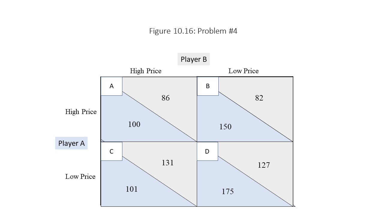
4. Consider the game in Figure 10.16:
Which players have dominant strategies in the game?
What is the outcome of the game?
Is the outcome of the game a dominant equilibrium?
Is it a Nash equilibrium?
5. Consider the game in Figure 10.17:
Which players have dominant strategies in the game?
What is the outcome of the game?
Is the outcome of the game a dominant equilibrium?
All the figures for unconcentrated, moderately concentrated, and highly concentrated industries are from the United States Census Bureau. “Manufacturing: Subject Series – Concentration Ratios: Share of Value Added Accounted for by the 4, 8, 20, and 50 Largest Companies for Industries: 2002.” 2002 Economic Census of the United States. Web. Accessed on May 11, 2018. ↵
For practical purposes, economists frequently calculate the HHI using the top 50 or top 20 firms in the industry even though technically all firms’ market shares should be included in the calculation. ↵
Reed, Brian. “Money in a Bottle: The Celebrity Scent Business.” National Public Radio. November 6, 2009. ↵
Samuelson and Nordhaus (2001), p. 212, present this case in a rather different way but arrive at the same result. ↵
See Sweezy, Paul. “Demand Under Conditions of Oligopoly.” Journal of Political Economy. Vol. 47, 1939. Pp. 568-573, which is also cited in Keat et al.’s (2013), p. 367, summary of the kinked demand model of oligopoly. ↵
Similar lists of factors that influence cartel formation are provided in many neoclassical textbooks. See Keat et al. (2013), p. 391-392, and McConnell and Brue (2008), p. 459-460. ↵
See Varian (1999), p. 476, for a similar graphical representation of the price leadership model. ↵
McConnell and Brue (2008), p. 464, emphasize this point. ↵


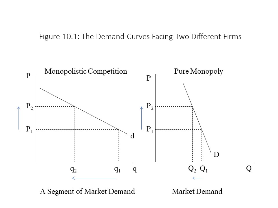 Figure 10.1 also shows the graph of a downward sloping demand curve facing a pure monopolist. Two important differences between the two graphs should be noted. First, whereas the demand curve facing the pure monopolist is the entire market demand curve, the demand curve facing the monopolistically competitive firm is only a segment of the market demand. Second, the pure monopolist tends to face a much more inelastic demand curve because no close substitutes for the product exist. Therefore, consumers will be much less responsive to price changes when the market is purely monopolistic because they cannot find good substitute products. A monopolistically competitive firm faces competition from firms that produce close substitutes. The widespread availability of substitutes suggests that the demand curve facing the monopolistically competitive firm will be far more elastic since consumers can respond to price changes more easily.
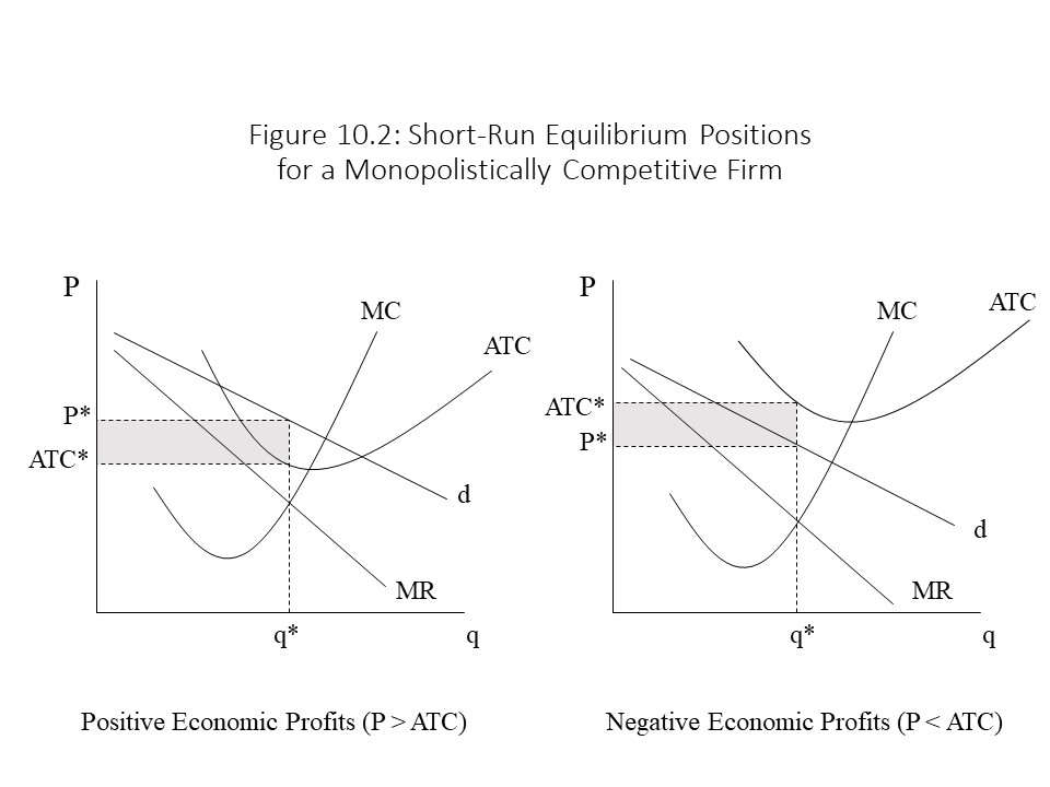 Depending on the relationship between the demand curve facing the firm and the unit cost curves, the firm may experience positive economic profits or negative economic profits in the short run. If the demand facing the firm is relatively high and unit costs are relatively low, then the firm will enjoy short run economic profits. If the demand facing the firm is relatively low and unit costs are relatively high, then the firm will suffer short run economic losses.
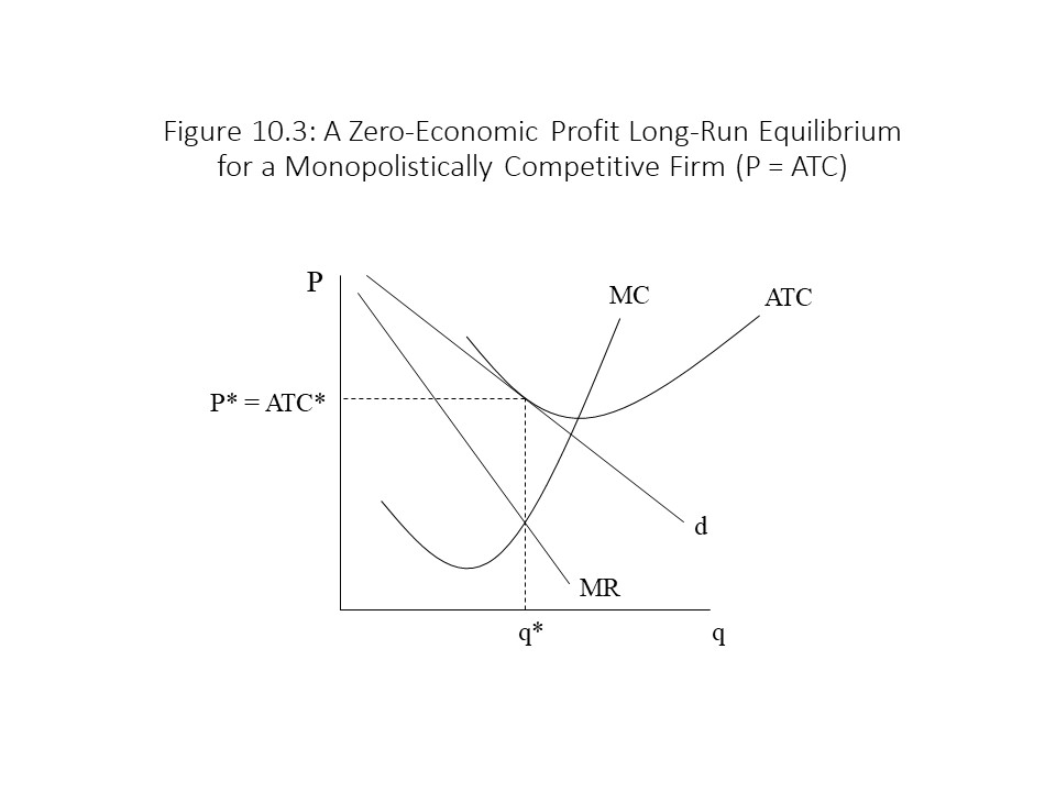 The reader should notice in Figure 10.3 that the demand curve facing the firm is just tangent to the ATC curve above the MR = MC intersection. At this point, price and ATC are the same and so economic profits are equal to zero in this case. How does this long run adjustment to zero economic profits occur? Two possible scenarios exist:
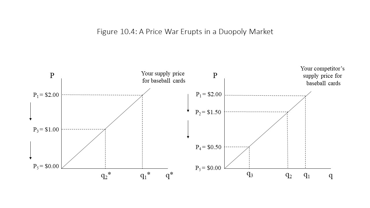
 Given the original price of P1, we need to determine the shape of the demand curve facing this firm. To derive the demand curve facing the firm, we ask what will happen if this firm raises its price above P1. Because we are assuming that firms think strategically, it is reasonable to expect that when this firm raises its price, the other firms will not follow with a price increase. By not following with a price increase, they can capture a larger share of the market. As a result, when this firm raises its price, its customers will react by purchasing the product from the firm’s competitors. That is, consumers will be very responsive to the price increase and the quantity demanded will fall significantly. In other words, the demand curve facing the firm is very elastic above the price of P1.
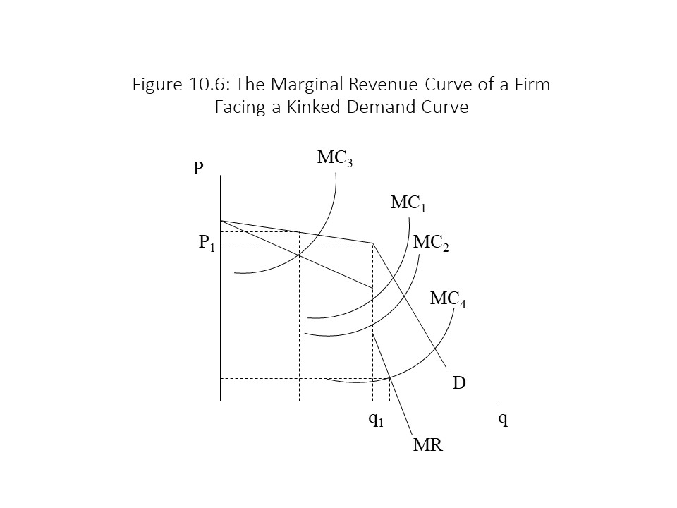 In Figure 10.6, the MR curve has a gap in it. The gap occurs at the same output level of q1 at which the kink occurs. This gap in the MR curve can be explained intuitively. Imagine that the firm is cutting the price at levels above P1. The MR is given by the flatter portion of the MR curve. Once the firm reaches P1, a substantial price cut is needed to sell one more unit. This large price cut causes the price to drop considerably for all other units sold and so the MR plummets, creating a gap in the MR curve. If the firm then continues to cut price along the inelastic portion of the demand curve, the MR falls steadily along the steeper portion of the MR curve.
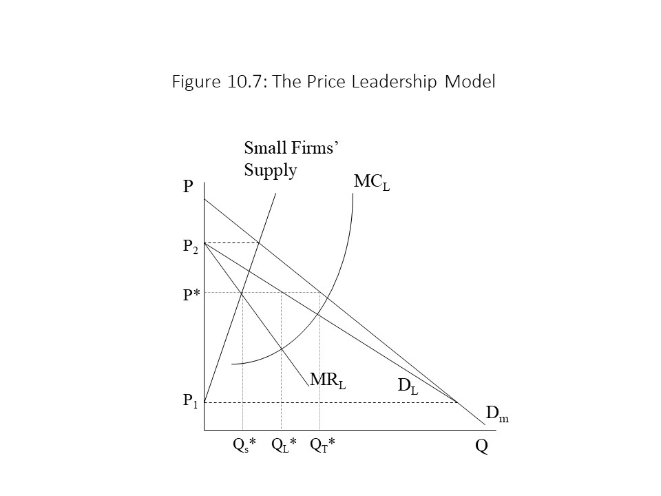 This graph is a bit involved and so we will discuss each piece before bringing all of them together to provide an explanation of how the market is divided when a price leader exists. First consider the market demand for automobiles (Dm). It is a downward sloping curve consistent with the law of demand. The small firms’ supply curve, on the other hand, is upward sloping consistent with the law of supply. As the price increases, the quantity supplied of the small firms rises because the higher price covers the higher marginal cost of production. If no other firms exist in this market, then the market will be perfectly competitive and the equilibrium price will be the competitive price of P2 where the supply of the small firms and market demand intersect.
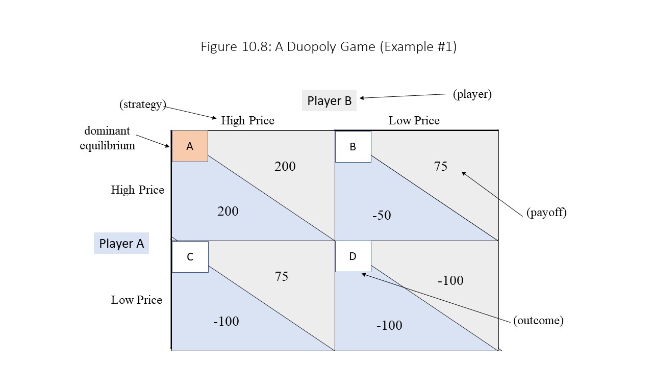
 As the Venn diagram shows, every dominant equilibrium is a Nash equilibrium but not every Nash equilibrium is a dominant equilibrium.
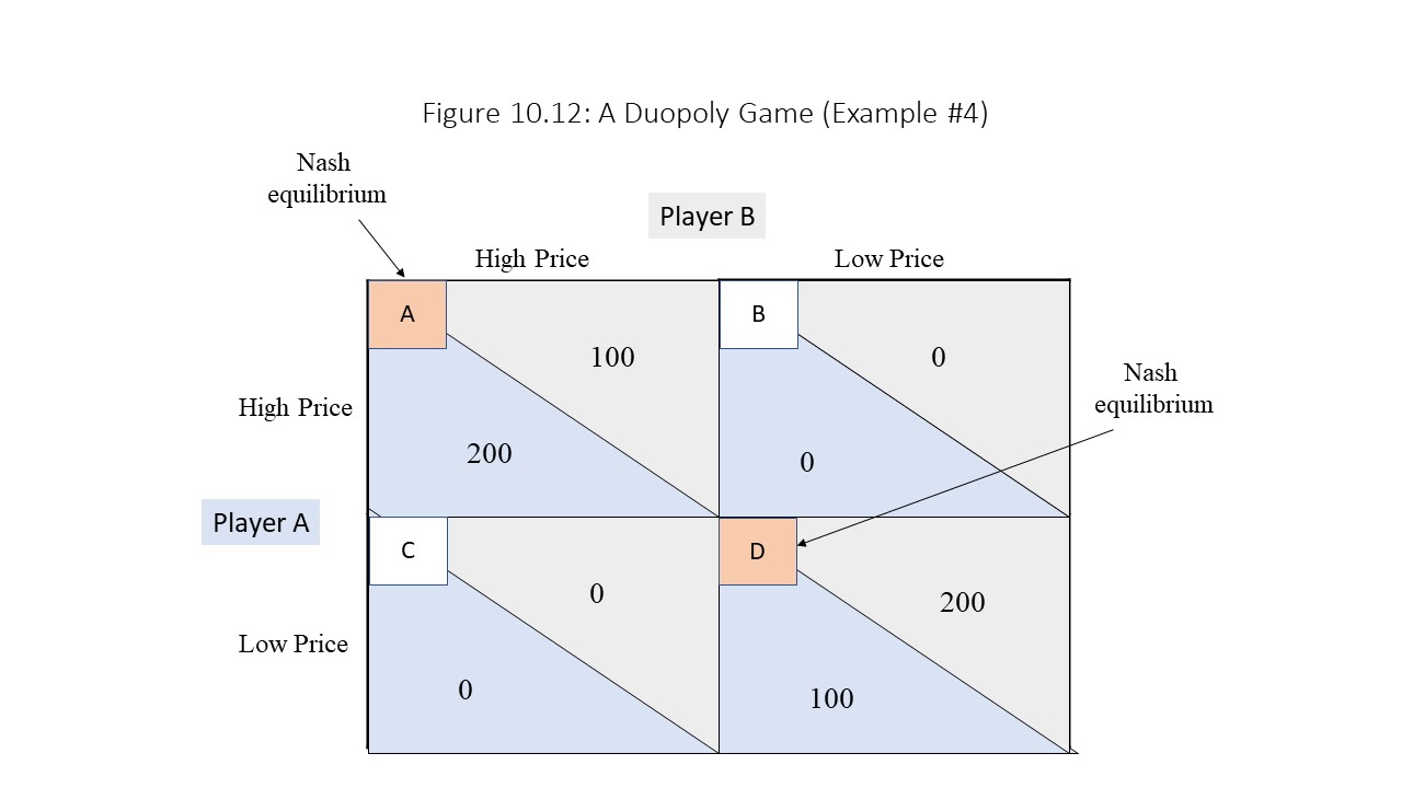
 Suppose the firm initially charges a price of $1.00 per unit and produces an output of 100 units. The ATC is $0.80 per unit in this case. The markup is $0.20 per unit. Notice that the firm has a small degree of excess capacity because it has not quite reached the lowest point on its ATC curve. The firm’s total profit in this case is $20 (= $0.20 per unit times 100 units). If a short run reduction in demand occurs, then the firm will maintain the price of $1.00 per unit but will reduce output from 100 units to 90 units. The firm keeps the price the same because this market is a fixprice market and short run changes in demand do not affect price. Post-Keynesian economists explain the reluctance to change price as stemming from firms’ fear that they might “spoil the market by damaging customer goodwill.” [21] The firm experiences an increase in excess plant capacity because it has reduced its output. Due to the failure to fully utilize its plant capacity and the gains from specialization, the per unit cost increases to $0.90 per unit. The markup thus falls to $0.10 per unit and profits decline to $9.00 (= $0.10 per unit times 90 units).
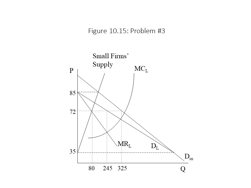 4. Consider the game in Figure 10.16: