
19: Theories of International Trade
- Last updated
- Save as PDF
- Page ID
- 46267

Goals and Objectives:
In this chapter, we will do the following:
- Explain the neoclassical theory of comparative advantage
- Analyze the limits to the terms of trade and the determination of the terms of trade
- Explore criticisms of the theory of comparative advantage
- Investigate the so-called New Trade Theory
- Examine the neoclassical approach to tariffs and quotas
- Consider radical theories of world trade
In this final part of the book, we explore key principles that will help us understand the operation of the world economy. This chapter concentrates on theories of international trade. The final chapter of the book considers theories of international finance. As in other chapters, much of the focus in the present chapter will be on the dominant neoclassical perspective. Unlike other economics principles textbooks, however, we will also consider criticisms of the mainstream theory of trade as well as radical theories that serve as alternatives to neoclassical trade theory. As before, these alternative theories of trade will provide us with a different perspective of the same material, but they will also deepen our understanding of mainstream trade theory.
The Ricardian Theory of Comparative Advantage
The theory of international trade that dominates mainstream neoclassical discourse today has its roots in a theory developed by David Ricardo in his 1817 book The Principles of Political Economy and Taxation. According to Ricardo, two nations can always gain from trade as long as each nation has a comparative advantage in the production of at least one commodity. That is, he argued that a richer nation might still gain from trade with a poorer nation even if it is a better producer of every commodity that the two countries produce. If the rich nation is relatively much better at producing one commodity than another, then it makes sense for the rich nation to specialize in the production of the commodity that it is relatively much better at producing. It can then engage in trade with the poor country, and both nations will be better off.
When Ricardo presented his theory, he did so using the classical labor theory of value. He assumed that one nation was absolutely better at producing both commodities. Within that framework, a nation has an absolute advantage if it can produce one unit of a commodity with less labor time than another nation. A nation has a comparative advantage in the production of a commodity, on the other hand, if its absolute advantage is relatively greater for that commodity. In that case, it should specialize in the commodity in which it has a comparative advantage. The other country should specialize in the production of the other commodity in which it will have a comparative advantage. Even though the poor country has an absolute disadvantage in the production of both commodities (more labor time is required to produce a unit of each commodity), it nevertheless has a smaller absolute disadvantage in the production of one commodity. The commodity in which it has a smaller absolute disadvantage is the one in which it has a comparative advantage.
Table 19.1 provides an example (like Ricardo’s original example) of two nations and the amounts of labor required to produce one unit of cloth and one unit of wine.
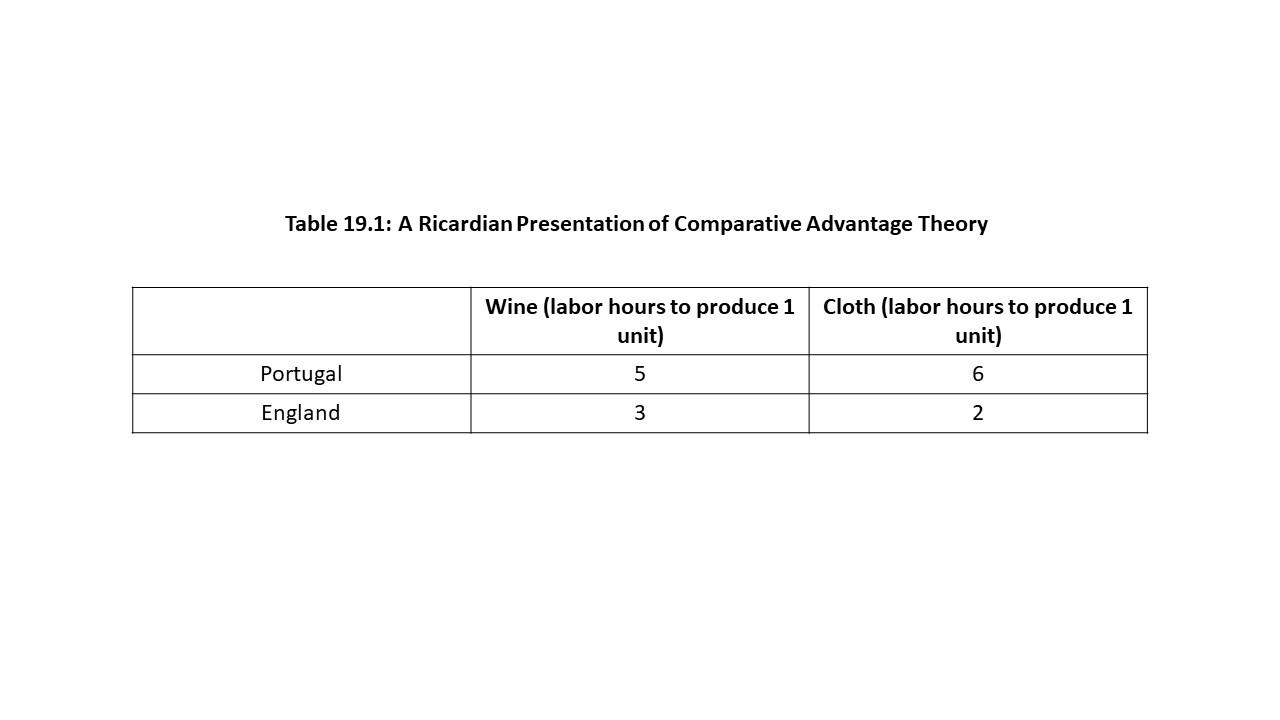
Table 19.1 shows that England has an absolute advantage in the production of both wine and cloth. That is, it requires absolutely less labor time in England to produce each commodity than in Portugal. At the same time, it requires 1 and 2/3 times as much labor time to produce wine in Portugal (= 5/3) as it does in England. Similarly, it requires 3 times the amount of labor time in Portugal to produce cloth (= 6/2). Therefore, Portugal’s absolute disadvantage is greatest in cloth production and so we should expect it to have a comparative advantage in wine production.
Similarly, England requires only 0.6 times as much labor time as Portugal to produce wine (= 3/5). England also requires only about 0.33 times as much labor time as Portugal to produce cloth (= 2/6). Again, we see that England can produce each commodity in less time than Portugal. Nevertheless, England’s absolute advantage is clearly greatest in the production of cloth. Therefore, England’s comparative advantage is in the production of cloth. In conclusion, England should specialize in cloth production, Portugal should specialize in wine production, and the two nations can trade to the benefit of each.
The Modern Theory of Comparative Advantage: The Case of Constant Opportunity Cost
Of course, mainstream economists have long since abandoned the classical labor theory of value. As a result, the Ricardian presentation is not the best way to represent the mainstream theory of international trade. Instead, we will return to the production possibilities model and consider an example in which Thailand and the United States produce both sugar (S) and corn (C). Each nation has a given production technology and given stocks of land, labor, and capital. We will also modify our earlier assumption from Chapter 2 that each nation experiences increasing marginal opportunity costs. The reader might recall that increasing opportunity cost arises because societies generally possess heterogeneous resources. Instead, we will assume that each nation possesses homogeneous resources that are equally well-suited to all lines of production and thus are easily transferrable from one industry to another. The assumption of homogeneous resources generates a pattern of constant marginal opportunity costs. Figure 19.1 shows the production possibilities for the U.S. and Thailand.
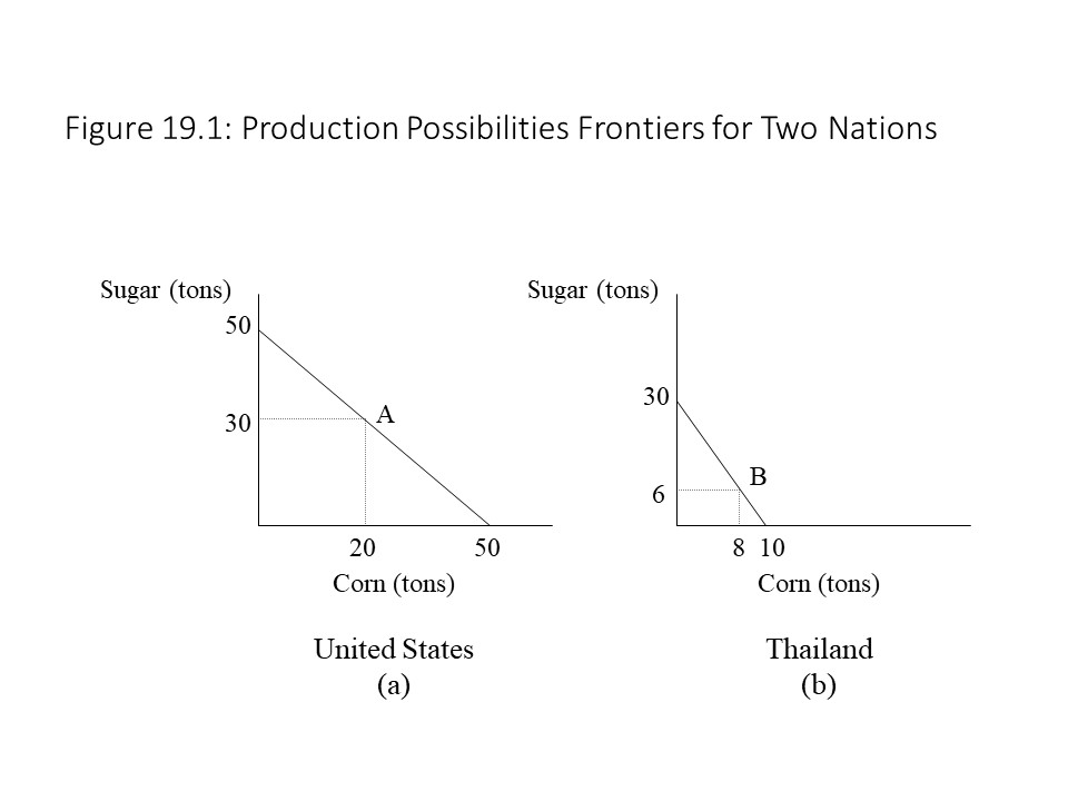 Because the slope of the production possibilities frontier (PPF) signifies marginal opportunity cost, the assumption of constant marginal opportunity costs explains the linear production possibilities frontiers of each nation. Points A and B on the two PPFs are included simply to provide examples of points that lie on the curves and to remind the reader that a nation may choose to be at any specific point on the PPF at a point in time by shifting resources across industries.
Because the U.S. has an absolute advantage in the production of both corn and sugar, the conclusion might be drawn that the U.S. should not trade with Thailand. If we recall Ricardo’s insight, however, that a nation only needs to have a comparative advantage for trade to be beneficial to it, then trade might still be worthwhile. To provide a definite answer to this question, we must introduce a modified definition of comparative advantage that is compatible with the production possibilities framework. It will be said that a nation possesses a comparative advantage in the production of a commodity if the marginal opportunity cost of production is lower for that nation than for another nation.
As mentioned previously, the marginal opportunity cost, also known as the domestic terms of trade, is reflected in the slope of the PPF. In the U.S., therefore, the marginal opportunity cost of corn is the following:
In other words, the opportunity cost of producing 1 unit of corn is 1 unit of sugar in the U.S. In Thailand, however, the domestic terms of trade are rather different. The marginal opportunity cost of producing corn in Thailand is the following:
That is, the marginal opportunity cost of producing 1 unit of corn in Thailand is 3 units of sugar. It should be clear that the marginal opportunity cost of producing corn is lower in the United States. In the U.S. it only costs 1 unit of sugar rather than 3 units as in Thailand. Therefore, the U.S. has a comparative advantage in the production of corn.
Thailand must have a comparative advantage in sugar production, but to verify this result, let’s consider the reciprocal of the slope. The reciprocal of the slope will allow us to see the marginal opportunity cost of producing 1 unit of sugar. For example, in the U.S. the marginal opportunity cost of sugar production is the following:
In other words, the marginal opportunity cost of 1 unit of sugar is one unit of corn. Similarly, we can write the marginal opportunity cost of 1 unit of sugar in Thailand as follows:
In other words, the marginal opportunity cost of 1 unit of sugar in Thailand is 1/3 units of corn. Therefore, the marginal opportunity cost of sugar production is lower in Thailand than in the United States since it costs 1 unit of corn in the U.S. but only 1/3 units of corn in Thailand to produce 1 unit of sugar. Thailand thus has a comparative advantage in sugar production.
In such examples, it will always be the case that if one nation has a comparative advantage in the production of a commodity, then the other nation will have a comparative advantage in the production of the other commodity. The only case in which a nation will not have a comparative advantage in the production of either commodity is the one in which the marginal opportunity cost is the same in the two nations. Trade in that case will not achieve anything that cannot be achieved domestically.
In this case, however, trade can benefit both nations. To understand how, we assume that each nation completely specializes in the production of the commodity in which it has a comparative advantage. That is, it is assumed that the U.S. shifts all its resources to the production of corn since it has a comparative advantage in corn production. Similarly, Thailand shifts all its resources to sugar production since that is where its comparative advantage lies. In Figure 19.1, the U.S. will produce at the horizontal intercept in (a), and Thailand will produce at the vertical intercept in (b).
Now that each nation is producing only one commodity, it will certainly want to trade a part of its production for the other commodity that is now only produced by its trading partner. The amount of the other commodity that each country will wish to import and the amount of its own commodity that it wishes to export will depend on the preferences of the consumers in each nation. Because the PPF only tells us about production possibilities and does not tell us about consumption possibilities, we do not possess enough information to address this question.
We are in a position, however, to draw some conclusions regarding the international terms of trade that will be established in the world market. The international terms of trade tell us how much sugar Thailand is willing to exchange for 1 unit of American corn. Its reciprocal tells us how much corn the U.S. is willing to exchange for 1 unit of Thai sugar. This international rate of exchange will be determined through a process of negotiation between the two nations. That is, competition in the marketplace will ultimately determine the price that emerges for each commodity.
Certain limits to the terms of trade exist though. To understand why such limits exist, consider the situation from Thailand’s perspective first. Would Thailand ever trade more than 3 units of sugar for 1 unit of corn? The answer is definitely “no.” According to its domestic terms of trade, Thailand can produce 1 unit less of corn and 3 units more of sugar by shifting resources from corn production to sugar production. It should never pay more in the world market than 3 units of sugar for 1 unit of corn since it is capable of that tradeoff at home. Similarly, the U.S. will never pay more in the world market than 1 unit of corn for 1 unit of sugar. According to its domestic terms of trade, the U.S. can shift resources from corn production to sugar production. If it does so, then it will gain 1 unit of sugar at the cost of 1 unit of corn. Since it can obtain 1 unit of sugar by only sacrificing 1 unit of corn at home, the U.S. will never be willing to pay more than 1 unit of corn in the world market.
This reasoning suggests that the domestic terms of trade serve as the maximum limits for the international terms of trade. Any international exchange ratio that falls within these limits, including the domestic exchange ratios themselves, is a possible outcome for the international terms of trade. For example, the international terms of trade might be the following:
In other words, in the world market, Thailand must pay 2 units of sugar for 1 unit of corn. This outcome is possible because the world price of corn lies in between the domestic prices (i.e., between 1 and 3 units of sugar). Similarly, taking the reciprocal allows us to consider the world price of a unit of sugar.
That is, 1 unit of sugar costs the U.S. 1/2 units of corn. The world price of sugar also lies between the domestic prices (i.e., 1/3 and 1 units of corn).
To visualize these limits to the terms of trade and this additional possible outcome for the international terms of trade, consider Figure 19.2.
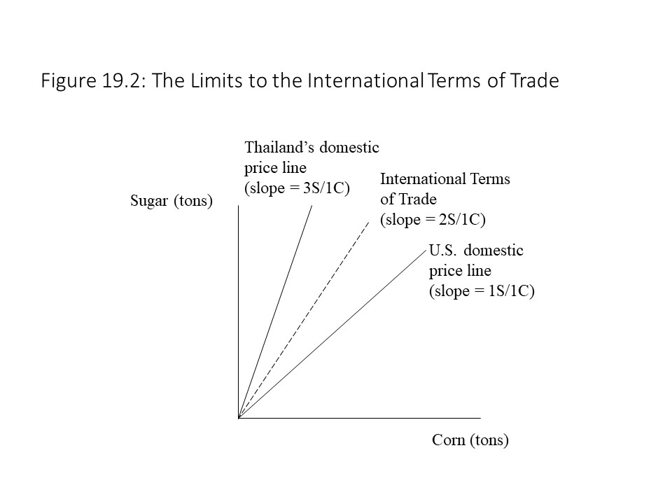 In Figure 19.2, the domestic marginal opportunity costs are represented as straight lines stemming from the origin. The negative signs of the slopes have been eliminated, but a tradeoff between the two commodities in each nation is implied. Because the domestic marginal opportunity costs are constant in each nation by assumption, these lines have constant slopes. The international terms of trade line must lie somewhere in between these extreme possibilities (although the extremes cannot be ruled out as possibilities for the established international terms of trade). If the international terms of trade line coincides with one of the domestic price lines, then that nation does not benefit from trade, and the other nation enjoys all the gains from trade. In this case, the international terms of trade line has a slope of 2 and thus it lies in between Thailand’s domestic marginal opportunity cost line, which has a slope of 3, and the U.S. domestic marginal opportunity cost line, which has a slope of 1.
The final step in this section is to determine what effect these specific terms of trade have on the consumption possibilities of Thailand and the U.S. Each nation is engaged in complete specialization in the production of the commodity in which it has a comparative advantage. Given the international terms of trade that have been established, each nation can export a part of its production in exchange for a definite amount of the other nation’s commodity. For example, the U.S. could hypothetically trade all 50 tons of corn for 100 tons of sugar at these specific terms of trade. Multiplying the numerator and denominator of the international terms of trade fraction by 50, the calculation may be completed as follows:
Because the U.S. can hypothetically reach this point of 100 tons of sugar as well as any other point along the straight line connecting these two points, we can add a trading possibilities frontier (TPF) to our earlier graph from Figure 19.1 (a). This graph is shown in Figure 19.3 (a).
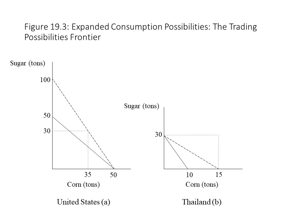
Similarly, Thailand can hypothetically export all its sugar for 15 tons of corn. Following a similar approach as the one used to obtain the TPF of the U.S., we can arrive at this result by multiplying the numerator and denominator of the international terms of trade fraction by 30:
Since Thailand can trade with the U.S. to reach any point on the straight line connecting these two points, it also has a trading possibilities frontier (TPF). Thailand’s TPF is represented in Figure 19.3 (b).
The major lesson from this analysis is that each nation can reach consumption combinations of the two commodities that lie outside their production possibilities frontiers. Neither nation has acquired more resources or more advanced production technologies, and yet each nation is able to consume more than before. Specialization and trade are what make this extraordinary result possible.
The careful reader might notice one little problem with the analysis. The maximum amount of sugar production in Thailand with complete specialization is 30 tons of sugar. Therefore, it is impossible for the U.S. to trade all its corn in exchange for 100 tons of sugar. Nevertheless, if it trades 15 tons of corn for 30 units of sugar, then it achieves a much higher level of consumption than what it can achieve without trade. The same holds true for Thailand. Aside from the complication of limited production in Thailand, each nation can achieve consumption possibilities that lie in between their PPFs and their TPFs. These results, therefore, suggest that international trade leads to mutual gains, and it is, therefore, the main reason why neoclassical economists argue so forcefully for free trade in the world market.
The Modern Theory of Comparative Advantage: The Case of Increasing Opportunity Cost
Now that we have a clear understanding of how nations may enjoy mutual gains from trade in the case of constant marginal opportunity costs, we can consider the case of increasing marginal opportunity costs. That is, we will assume that nations have production possibilities frontiers like those we considered in Chapter 2. Again, the underlying assumption that gives rise to this pattern of increasing opportunity cost is the assumption of heterogeneous resources.
Let’s assume that the U.S. and Thailand have the PPFs shown in Figure 19.4., and that each nation is producing at the points identified on their PPFs in the figure.
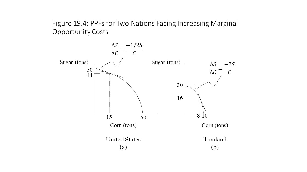
In this example, the U.S. is producing 15 tons of corn and 44 tons of sugar in autarky. Autarky refers to a closed economy, or an economy that does not engage in trade relationships. That is, it neither imports nor exports commodities. The slope of the tangent line drawn to the PPF at that point tells us the marginal opportunity cost of corn production. Let’s assume that this slope is -0.5S/C. That is, the opportunity cost of producing 1 unit of corn is 1/2 unit of sugar in the U.S. as shown in Figure 19.4 (a). Similarly, Thailand is producing 8 tons of corn and 16 tons of sugar. The marginal opportunity cost of producing corn is also determined by the tangent line that just touches the curve at that point. Let’s assume that the slope is -7S/1C. That is, the opportunity cost of producing 1 ton of corn in Thailand is 7 tons of sugar as shown in Figure 19.4 (b). It should be clear that the U.S. has a comparative advantage in corn production. Thailand would then have a corresponding comparative advantage in sugar production.
As before, each nation will specialize in the commodity in which it has a comparative advantage. That is, the U.S. will begin shifting resources towards corn production, and Thailand will begin shifting resources towards sugar production. Something interesting happens in this case, however, that is very different from the case of constant opportunity cost that we considered before. As the U.S. begins producing more corn, the marginal opportunity cost of corn production begins to rise. This increase occurs because less suitable resources must be increasingly relied upon as the best resources for sugar production are transferred to corn production. At the same time, Thailand’s increased production of sugar causes the marginal opportunity cost of sugar production to rise for the same reason. Eventually, the marginal opportunity cost of corn production in each nation will be the same. That is, the domestic terms of trade will be exactly the same in each nation. At this point, the specialization ceases because neither nation will have anything to gain from further specialization. This situation is depicted in Figure 19.5.
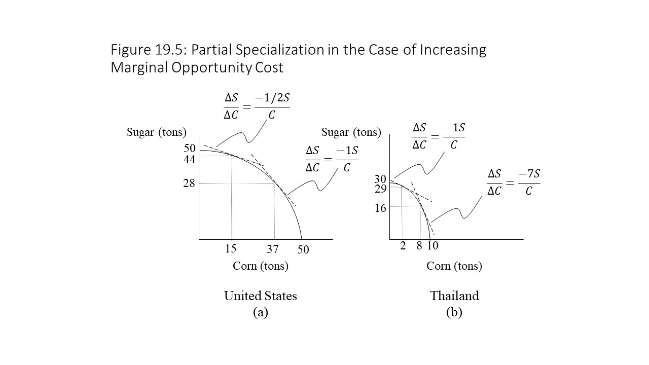
As Figure 19.5 shows, the two nations cease to increase their degrees of specialization once the domestic marginal opportunity costs in each nation are equal to 1 ton of sugar for each ton of corn. That is, once the slopes of the PPFs in each nation are equal to -1S/C, then the domestic prices in each nation are the same. The interesting result, in this case, is that each nation only pursues partial specialization. That is, each nation will not completely specialize in the production of the commodity in which it has a comparative advantage because its comparative advantage would then become a comparative disadvantage.
Once the marginal opportunity costs of the two nations have become equal, the limits to the terms of trade become identical for the two nations. Therefore, the international terms of trade must be the same as the domestic terms of trade once partial specialization is achieved. Unlike in the case of constant opportunity cost, the case of increasing opportunity cost leads to a unique outcome for the international terms of trade. Each nation partially specializes in one commodity and then exports some of that commodity in exchange for the commodity in which the other nation partially specializes.
As it turns out, we have only discussed part of the story. Demand also plays a role in determining the equilibrium terms of trade. To provide the complete picture, we would need an additional analytical tool to represent consumer preferences in each nation. Let’s just move to a graph that will allow us to see how both supply and demand contribute to the determination of the equilibrium terms of trade. Figure 19.6 shows what are referred to as offer curves in mainstream trade theory, and it has its roots in the theory of international prices developed by John Stuart Mill.[1]
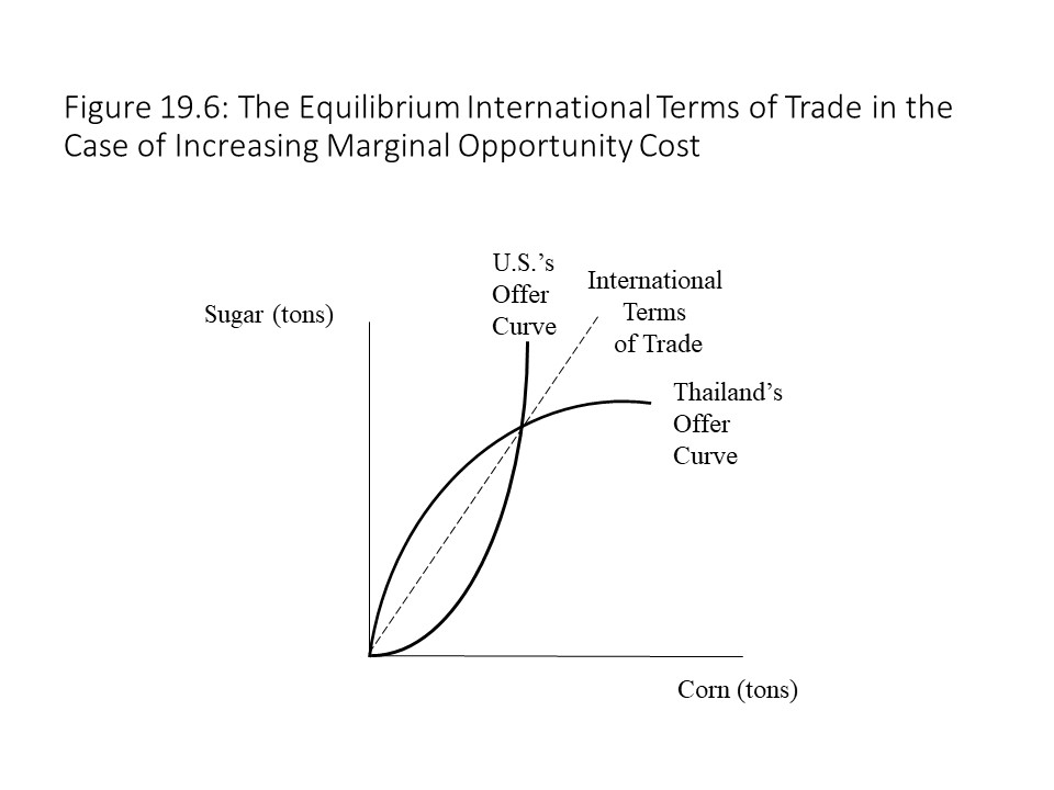 The offer curve of the U.S. in Figure 19.6 shows how much corn the U.S. is willing to supply to Thailand for a given quantity of sugar. As the U.S. specializes more in corn, the marginal opportunity cost of corn production rises, which contributes to the rapid increase in the quantity of sugar required in exchange. Consumer preferences also play a role and so the offer curve reflects the impact of both production cost and consumer demand. Thailand also has an offer curve. Its offer curve shows how much sugar it is willing to supply in exchange for a given quantity of corn from the U.S. Its requirement of corn increases rapidly as well, as its production of sugar rises, as shown in Figure 19.6, which is also due to the rising marginal opportunity cost of sugar and the strength of demand.
In the above equation, PC represents the price of corn, C represents the quantity of corn, PS represents the price of sugar, and S represents the quantity of sugar. Hence, the value of corn exported must equal the value of sugar imported in the U.S., and similarly, the value of corn imported must equal the value of sugar exported from Thailand. If we rearrange the equation, we obtain the following result:
This equation shows that the price of corn relative to the price of sugar (i.e., the relative price ratio) may be represented as the slope of a ray drawn from the origin, which may be calculated as the ratio of S to C at any point along that ray. If the ray becomes steeper, then the relative price of corn has risen. If the ray becomes flatter, then the relative price of corn has fallen. In addition, the nation’s trade is balanced if it operates on this ray.
Now suppose that the international terms of trade are given by the line TOT1 in Figure 19.7.
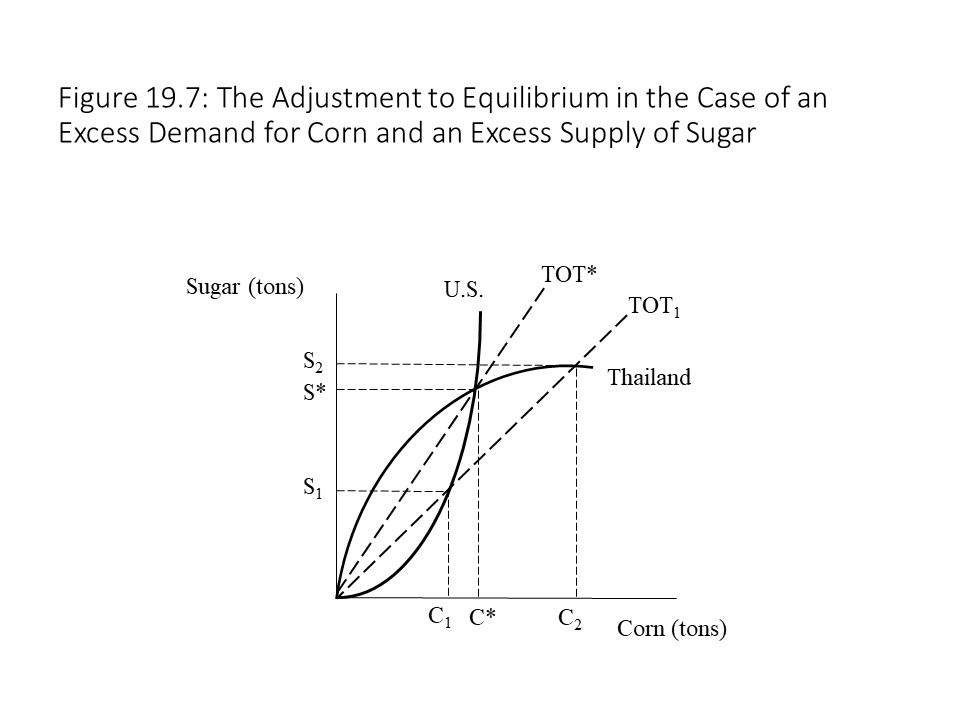
In this case, if the U.S. produces and offers C1 amount of corn in the market in exchange for S1 amount of sugar and succeeds in doing so, then its trade will be balanced. The problem, however, is that Thailand will offer S2 amount of sugar and wish to import corn of C2. In other words, a large excess demand for corn will exist. Similarly, a large excess supply of sugar will exist. As a result, the relative price of corn will rise, and the relative price of sugar will decline. As the relative price of corn rises, the terms of trade line becomes steeper and moves in the direction of the equilibrium terms of trade line (TOT*) at the intersection of the two offer curves.
Next suppose that the international terms of trade are given by the line TOT2 in Figure 19.8.
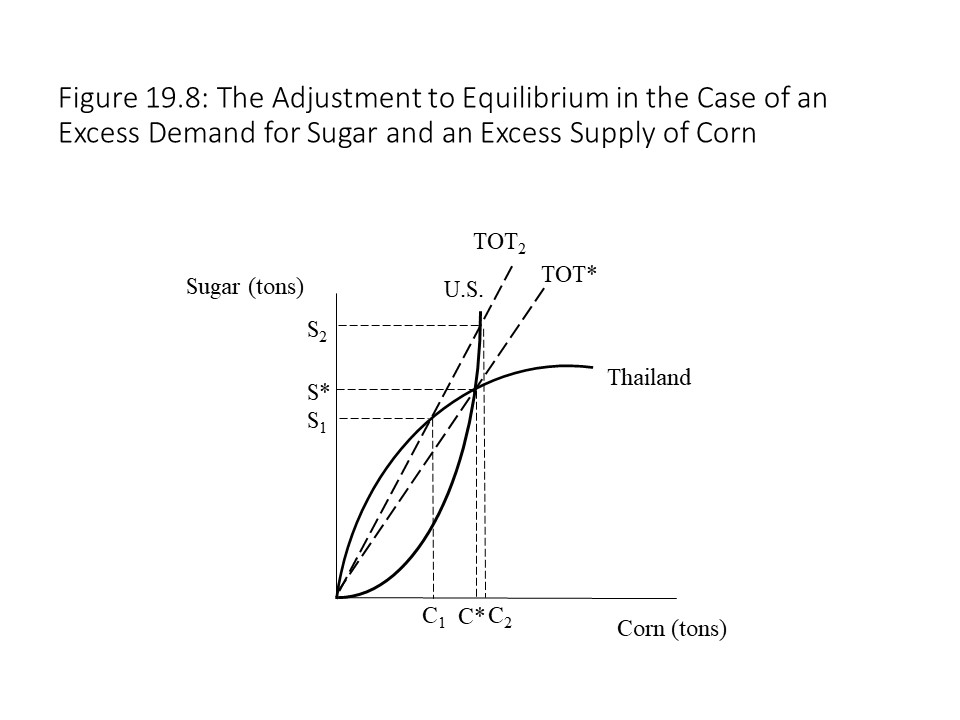 In this case, Thailand produces and offers S1 amount of sugar and wishes to import C1 of corn. If it succeeds then its trade will be balanced. The problem this time is that the U.S. is offering a great deal more corn (C2) and wishes to buy S2 tons of sugar, which is much more than Thailand wishes to export. As a result, an excess demand for sugar exists and an excess supply of corn exists in the world market. As a result, the relative price of sugar will rise and the relative price of corn will fall. As the relative prices change, the ray from the origin, which represents the international terms of trade, becomes flatter. It is only when the ray passes through the point of intersection of the two offer curves that each nation is balancing its trade, which is reflected in the fact that each nation is operating on the terms of trade line and its offer curve. Trade has become balanced due to international prices responding to the competitive pressures of supply and demand in the world market.
Criticisms of the Neoclassical Theory of Comparative Advantage
The theory of comparative advantage remains the foundation of the neoclassical theory of international trade to this day. It is more than just a theory of how nations engage in trade with one another. It is also an ideological defense of free trade. That is, economists reject any kind of government restrictions on international trade on the grounds that such restrictions undermine the potential for the mutual gains from trade to be realized. Because the theory of comparative advantage is the foundation of the free trade theory that most economists advocate, it is important to consider heterodox critiques of the theory to determine whether they have any merit.
One argument that is made in favor of free trade is that a nation’s exports generate sufficient revenue to finance the purchases of imports. Hence, trade should be balanced. It is important to note, however, that just because a nation recently sold commodities does not mean that it must immediately buy commodities from another nation. A trade surplus may persist if the nation does not purchase imported commodities. Meanwhile the other nation has purchased commodities but is unable to sell. It will, therefore, experience a trade deficit. If it finances its purchases using foreign currency reserves and those reserves begin to run out, then the result may be a currency crisis. The argument that imports can always be financed by exports is rather similar to the argument that whenever commodities are produced, enough income is paid to the factors of production to ensure the purchase of those commodities. We identified this claim in Chapter 13 as Say’s Law of Markets. The problem, of course, is that just because incomes have been received does not guarantee that they will be spent any time soon. If enough income is saved, then the result is a glut of commodities. In both examples, gaps between the time income is received and the time it is spent create the possibility of economic crises.
The problems with mainstream trade theory go far beyond this specific issue and relate to the assumptions underlying the theory of comparative advantage. In his book Free Trade Doesn’t Work (2009), Ian Fletcher provides a detailed account of eight hidden assumptions that form the basis of the theory.[2] Fletcher argues that exposing the assumptions reveals the flaws inherent in the theory. This section and the next section provide a brief overview of Fletcher’s insights.[3]
The first hidden assumption that Fletcher identifies is the assumption that trade is sustainable.[4] To finance its imports, a nation may not be exporting commodities but rather assets.[5] If it sells bonds, for example, then its debts may accumulate to the point where the future interest payments associated with that debt interfere with future capital investments and/or consumption. A nation may also specialize in the production of a non-renewable natural resource because it has a comparative advantage in its production.[6] Mutual gains from trade might exist in the short run, but in the long run, its exports will deplete its natural resource base to the point where it might experience a massive economic crisis. Fletcher offers Nauru as an example of an island nation that exported large quantities of guano, which is used for manufacturing fertilizer, from 1908 to 2002.[7] The economy boomed in the 1960s and 1970s. When the guano ran out, the economy collapsed. Middle Eastern nations that are heavily dependent on exports of petroleum might experience similar problems of economic dislocation as their oil reserves are depleted.[8]
The second hidden assumption that Fletcher identifies is the assumption that no externalities exist.[9] Ideally, the prices that emerge in the world market should reflect all costs and benefits associated with the production and consumption of the commodities traded. If third parties are affected by the production or consumption of the products, either positively or negatively, then positive or negative externalities exist and the commodities are either under-produced or over-produced, as discussed in Chapter 3. For example, if a production process leads to air pollution, then efficiency requires that the commodity produced be priced high enough to cover the costs to third parties who are then compensated for the harm done to them. If this corrective action is not taken, then the commodity will be produced in quantities that are too large, and the price will be too low.
The third hidden assumption is that factors of production are easily transferred from one industry to another.[10] Consider our earlier example involving constant opportunity costs in which the U.S. completely specialized in corn production and Thailand completely specialized in sugar production. Complete specialization requires a nation to shift all its resources away from the production of the commodity in which it has a comparative disadvantage. The problem is that transferring resources may not be an easy task to accomplish. Factories need to be converted to an entirely new type of production. Workers who may be considerably skilled at producing one type of commodity must now produce an entirely different commodity. The training involved may be expensive and time-consuming. The result very well may be unemployment of labor and production capacity that is not used for a long time. The theory of comparative advantage is entirely static. That is, the passage of time is not taken into account. Therefore, this problem is not obvious when considering movements along a production possibilities frontier, but the problem will be very real for workers and factory owners when cheaper imports begin to enter their nation.
The fourth hidden assumption is that international trade unambiguously raises the welfare of everyone in the nation.[11] After all, each nation can import the commodity it desires at a lower price. In our constant opportunity cost example, the U.S. acquires sugar at a lower price than it could domestically, and Thailand acquires corn at a lower price than it could domestically. We also saw that both nations enjoyed trading possibilities frontiers that lie beyond their production possibilities frontiers. The problem, however, is that with some industries contracting and other industries expanding, the gains are not equally shared. In fact, some workers and capital owners will lose income as a result of trade. A net gain for society as a whole does occur, however, because the winners gain more than the losers lose. According to the Kaldor-Hicks criterion, as long as the winners can hypothetically compensate the losers, the situation represents an improvement (even if the compensation does not actually occur). Nevertheless, the welfare gain for the nation may not be shared by all, and so this criticism is worth considering when evaluating the comparative advantage model.
The fifth hidden assumption is that capital is not internationally mobile.[12] If capital is able to leave the nation and seek more productive opportunities in other nations, then the comparative advantage model does not apply. Remember that the nation’s resource stocks determine the position of its PPF. If a nation begins to lose capital as trade begins, then its PPF will shift inwards. None of the results we discussed earlier would apply in such a situation. When Ricardo first developed the theory of comparative advantage, the assumption of capital immobility was more realistic. In the modern world, capital is highly mobile and so the argument is that the comparative advantage model does not apply very well today.
The sixth hidden assumption is that short-term efficiency is compatible with long-term economic growth.[13] As a static model, the theory of comparative advantage has nothing to say regarding the long-term growth prospects of the nation. Indeed, it is possible that a nation that chooses to specialize in the production of a commodity in which it has a comparative advantage might become permanently stuck producing a commodity that does not promote long-term economic growth. The original example that Ricardo used involved Britain’s specialization in textile production and Portugal’s specialization in wine production. As Fletcher points out, the British textile industry promoted technological change with the development of steam engines and sophisticated machine tools.[14] Wine, on the other hand, was produced using traditional methods that did not encourage innovation or productivity improvements.[15] Although Portugal may have benefited from specializing in wine production at the time, it is now the poorest nation in Western Europe.[16] Its goal of static efficiency appears to have been achieved at the expense of its long term growth prospects.[17]
The seventh hidden assumption is that trade does not induce adverse productivity growth abroad.[18] It is possible that trade might promote foreign industries to the point where their comparative advantage begins to change. In that case, the commodities that the foreign nation previously supplied are no longer supplied. The example that Fletcher gives is that of Japan in the 1950s and 1960s.[19] As the Japanese economy boomed, it transitioned from providing the U.S. with cheap manufactured commodities to those that required more sophisticated manufacturing processes.[20] This problem is not as serious as some of the others mentioned because the nations still gain from trade. The argument appears to be that the importing nation might not gain as much as previously.
Development s in New Trade Theory: The Potential Impact of Economies of Scale
Ian Fletcher’s eighthhidden assumption is that no economies of scale exist in production.[21] This assumption leads to a discussion of what has become known as New Trade Theory. One of the major contributions to New Trade Theory was made by Ralph Gomory and William Baumol in their book Global Trade and Conflicting National Interests (2000).[22] In their book, Gomory and Baumol assume that economies of scale in production do exist.[23] Therefore, they depart from the traditional assumption implicit in the theory of comparative advantage that no scale economies exist.
To understand how scale economies lead to different theoretical results, we need to understand what Gomory and Baumol mean by “retainable industries.” Retainable industries are industries that a nation captures and retains due to a cost advantage stemming from economies of scale.[24] To capture such industries, the nation must be the first to achieve a large enough volume that such low per unit production costs cannot be easily matched by competitors in other nations.[25] What is interesting about retainable industries is that a nation might capture one even if another nation would turn out to be a superior producer if it managed to reach the same large volume of production as its competitor. The reason that the superior producer fails to do so is that scale economies serve as a barrier to entry, preventing the potential competitor from entering the market. Fletcher refers to this possibility as the lockout phenomenon.[26]
Figure 19.9 provides an example involving Japan and China where each nation enjoys economies of scale in production as reflected in the downward slope of their average cost (AC) curves.[27]
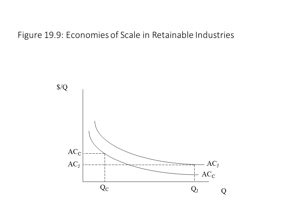 It should be clear from Figure 19.9 that China is the superior producer. At any level of output, China has a per unit production cost that is below Japan’s per unit cost. Because Japan entered the industry much earlier, however, its larger production level of QJ allows it to produce at a much lower per unit cost than China, which produces an output level of QC. Clearly, if China expanded production to match Japan’s output, then its unit cost would be lower and it would capture the industry, but because its unit cost is higher, firms will not be able to compete and its superior efficiency will not be realized. In this case, the industry is a retainable industry for Japan, and the world economy loses out on an opportunity to produce the product at a lower unit cost. That is, free trade may not produce the best result for the world economy because many efficient producers will be locked out.
Fletcher draws upon this theory to explain why Bangladesh exports many T-shirts but few soccer balls while Pakistan exports many soccer balls but few T-shirts.[28] That is, economies of scale allowed these nations to capture specific industries, and those nations that achieve large production volumes first are the most likely to retain those industries.
It might seem that a nation’s best trade strategy in a world of scale economies is to capture as many retainable industries as possible by increasing production rapidly to drive down unit costs.[29] Fletcher explains that a nation should pursue such a strategy but only up to a point.[30] That is, if a home nation captures too many retainable industries, then it might actually prevent other nations from producing and exporting commodities to the point where it misses out on the superior efficiency of its competitors.[31] It might also leave other nations impoverished and unable to buy the exports of the home nation.[32] Furthermore, the home nation might find its own resources to be spread too thinly.[33] To see how a nation might go too far, consider the graph in Figure 19.10.[34]
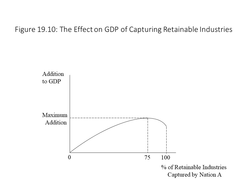
Figure 19.10 shows what happens to a nation’s GDP as it captures a larger percentage of the world’s retainable industries. Its GDP increases with the capture of more industries but only up to a point. Beyond that point, its GDP begins to fall for the reasons stated.
The analysis has a startling implication for trade theory. It suggests that trade is not always a positive sum game.[35] A positive sum game refers to a situation in which all players may gain without anyone losing. The theory of comparative advantage suggests that competitive interaction in the international marketplace is a positive sum game. The economic pie is made larger as both nations experience expanded consumption possibilities. The potential for a negative impact on income distribution is not explicitly captured in the model and so it appears to be a positive sum game. A zero-sum game, on the other hand, occurs when one player may gain but only at the expense of another player. The suggestion of New Trade Theory is that international trade is sometimes a zero-sum game in which one nation gains at another nation’s expense. This perspective directly contradicts what mainstream economists have long argued about the mutual benefits from international exchange.
To see how the assumptions of New Trade Theory generate this interesting result, consider Figure 19.11.[36]
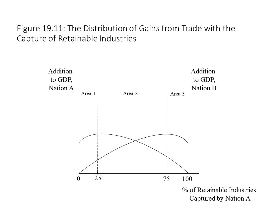
In Figure 19.11, we see how each nation’s GDP changes as it captures or loses retainable industries. As nation A increases its share of retainable industries in Area 1, its GDP increases. Notice that nation B also experiences an increase in GDP as it loses retainable industries. The reason is that nation B would be overreaching if it acquired such a large percentage of retainable industries. Giving up some of these industries to nation A actually benefits nation B. Both nations gain from trade, and this result is consistent with what neoclassical economists have long argued about the mutual gains from international trade.[37]
We discover a similar result in Area 3. In Area 3, nation A experiences a loss of GDP as a result of overreaching. It has captured so many retainable industries from nation B that its GDP begins to fall. Therefore, Nation A will prefer to capture fewer industries. Nation B, on the other hand, will prefer to capture more retainable industries because it has not yet captured many. In doing so, its GDP will rise so it will happily acquire the retainable industries that Nation A is willing to sacrifice. We see another example of a positive sum game and of mutual gains from trade, consistent with the traditional neoclassical conclusions about free trade.
It is in Area 2 where we see a very different result. In Area 2, Nation A gains from capturing more retainable industries. Nation B, however, also wants retainable industries and so any gains in GDP for Nation A must come at the expense of Nation B. Similarly, any gains in GDP for Nation B must come at the expense of Nation A in this region. This area is characterized by mutual conflict rather than mutual benefit.[38] A theory of international trade that suggests trade is a zero-sum game is one that contrasts very sharply with conventional trade theory.
This New Trade Theory suggests that foreign productivity growth might lead to a loss of GDP, sending the gains from trade into negative territory.[39] It also suggests that the consequences of trade are rather complicated, sometimes leading to mutual benefit and sometimes leading to conflict.[40] Fletcher’s policy conclusion is that free trade should be the rule in Ricardian industries in which no economies of scale are present.[41] Because of the existence of retainable industries, however, he favors something called rational protectionism.[42] That is, free trade should be the rule in Ricardian industries, but protectionism should be used in the case of retainable industries. For example, subsidies should be given to industries that are relatively new but in which large scale economies exist. Such subsidies will allow firms to break into industries in which the low unit costs of foreign rivals are likely to keep them out.[43] Infant industry tariffs are another option to protect domestic industries from foreign competition so that they have an opportunity to grow and take advantage of scale economies.[44] Infant industry tariffs are taxes on imported commodities aimed at protecting fledgling domestic industries.
Although he advocates rational protectionism, Fletcher does acknowledge the difficulties associated with such a policy stance. One of the main challenges is knowing which industries to target.[45] Another difficulty is that many modern corporations have become multinational in scope. It may be difficult to identify the home nation in which case it is not clear how such firms would even fit into this analysis.[46]
The Neoclassical Critique of Protectionist Policies : Import Tariffs and Quotas
In addition to the neoclassical theory of comparative advantage, mainstream economists also rely on partial equilibrium analyses to defend the claim that protectionist policies reduce social welfare by undermining efficiency. To understand why, let’s consider the case of a small nation that has a domestic supply and demand for a specific good. Furthermore, let’s assume that it can import all it wants at the world market price (Pw). This situation is depicted in Figure 19.12.
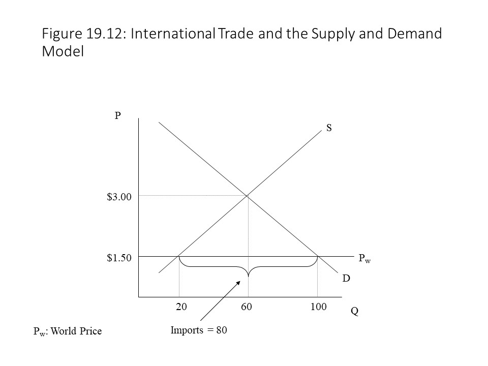
In this market, the equilibrium autarky price is $3.00 per unit, and the equilibrium quantity exchanged is 60 units. Because trade is permitted, however, and the world price is only $1.50 per unit, the domestic producers will only produce and sell 20 units. At that price, the remaining 80 units of the 100 units demanded will be imported. Free trade, therefore, allows the small nation to consume a larger quantity of the good and at a lower price than in the case of autarky. This result is basically consistent with the conclusion of comparative advantage theory.
The reader should also recall that the welfare of the consumers in the market can be measured using consumers’ surplus. In Figure 19.12, consumers’ surplus is equal to the area below the market demand curve and above the world price line at $1.50. In this case, no producers’ surplus exists because the world supply curve coincides with the world price line and so the price received by producers is just enough to cover production costs. Therefore, the large triangle representing consumers’ surplus also represents the total surplus or total welfare of all market participants.
The next question that we might consider is what will happen if the government decides to impose a tariff on imports. An import tariff is simply a tax on imported goods. In this case, the tariff is assumed to take the form of a tax per unit of physical product. For example, if the tariff is $0.75 per unit and the world price is $1.50 per unit, then the producers in the rest of the world must simply add $0.75 to the world price. The new world price then becomes $2.25 per unit. This situation is depicted in Figure 19.13.
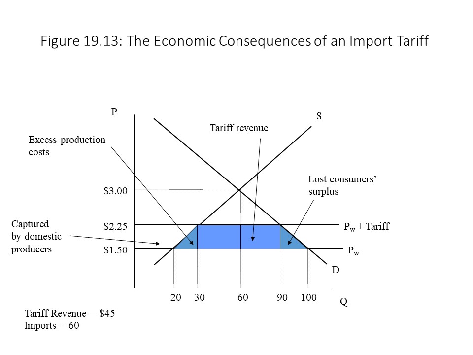
In Figure 19.13, we see that the effect of the higher price is to reduce the quantity demanded of the product domestically from 100 units to 90 units. In addition, the higher price encourages domestic producers to produce and sell 30 units of the good rather than the 20 units previously sold. Imports thus fall to 60 units, which is the difference between the quantity demanded and the quantity domestically supplied.
In terms of the impact on social welfare, we need to consider what happens to consumers’ surplus due to the tariff. In Figure 19.13, all the areas labeled represent lost consumers’ surplus due to the higher world price. One of these regions, however, is captured by domestic producers in the form of producers’ surplus, which they receive now that they are able to charge a higher price as well. This gain is the portion above the domestic supply curve (and between the old and new prices). The portion that is below the domestic supply curve from units 20 to 30 (and above the old price) represents excess production costs that the higher world price allows the domestic producers to incur. In other words, the higher world price allows the domestic producers to produce inefficiently. Because it does not represent producers’ surplus and it is lost as consumers’ surplus, it therefore represents a deadweight loss to society.
An additional deadweight loss to society that results from the tariff derives from the reduction in quantity demanded that occurs when the world price rises. Because consumers consume 10 fewer units as a result of the tariff, it is not possible for any consumers’ surplus to be realized on these units. Furthermore, since the units are not produced, producers cannot capture these gains, and the welfare simply vanishes. The final portion that must be considered is the rectangle in the middle, which represents tariff revenue. The base of the rectangle represents the quantity of imports, which in this case is 60 units. The height represents the tariff per unit of $0.75. If we multiply the tariff per unit times the quantity of imports, we obtain the total tariff revenue of $45 (= $0.75 per unit times 60 units). This portion of the lost consumers’ surplus is captured by the government and so it is not a deadweight loss. The government has the power to use this revenue to provide services for the nation’s citizens and so it does not necessarily lead to a shrinking of the economic pie. Overall, however, the economic pie shrinks due to the excess production costs that protected firms are able to incur and the reduction in quantity demanded resulting from the higher world price.
One final protectionist policy that we might consider is an import quota. An import quota is simply a quantitative limit on the amount of a good that may be imported into a nation. For example, the government might set an import quota of 60 units. Therefore, the maximum quantity that may be imported of the product is 60 units. What the quota means is that the total supply of the product will now be equal to the U.S. domestic supply plus the quota amount. That is, the domestic supply curve will shift to the right by the amount of the quota, as shown in Figure 19.14.
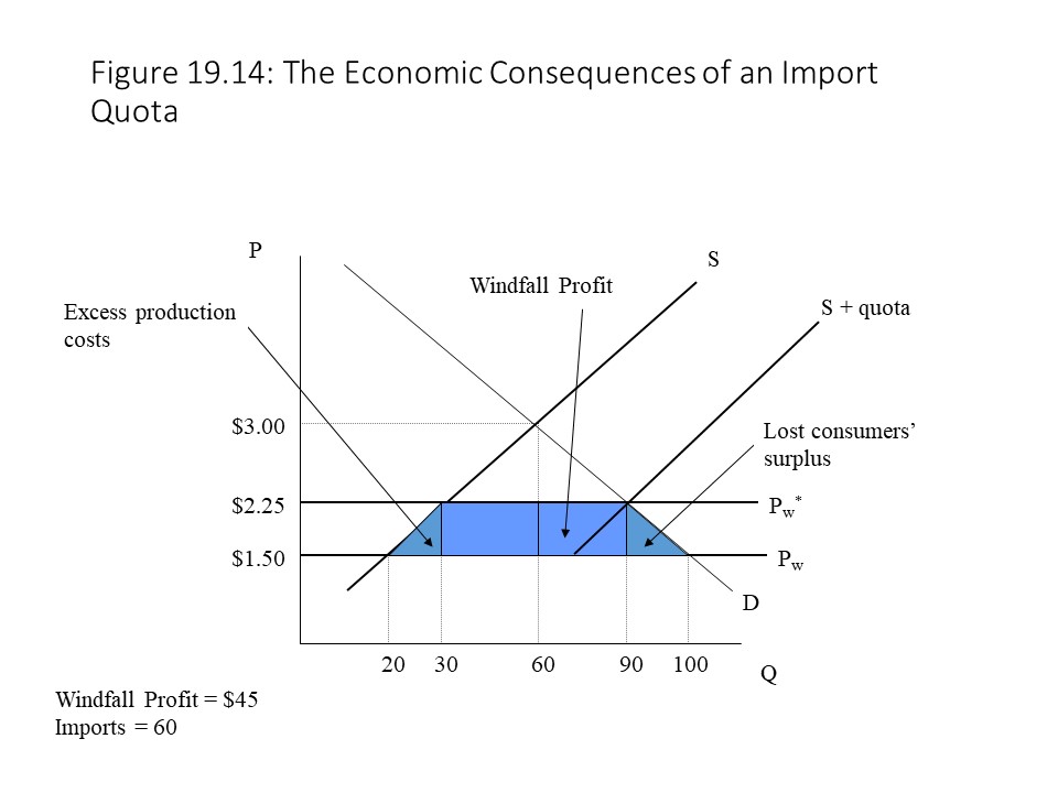
The intersection between the new supply curve and the demand curve gives us an equilibrium price of $2.25 and an equilibrium quantity exchanged of 90 units. The result in this case looks very much like the result we obtained in the case of an import tariff. In fact, the new world price and the quantity of imports are the same as in the case of the tariff. The welfare effects are also similar. We see that more domestic producers produce the commodity at a higher cost thanks to the restriction on imports, which makes possible the higher price. We also see that the quantity demanded drops leading to a lower consumers’ surplus. Both of these effects contribute to the deadweight loss of the policy.
As before, the domestic producers do gain producers’ surplus at the expense of consumers. The one consequence of the import quota that makes this case rather different from the import tariff is the portion of lost consumers’ surplus represented with the rectangle. Because the government does not collect a tax but simply limits the quantity of imports, who collects this extra revenue from the sale of the product? As Robert Carbaugh explains, the answer depends on whether foreign exporters or domestic importers have greater market power.[47] For example, if the foreign exporters collude, then they can demand a price of $2.25 per unit from domestic importers. The exporters will then gain the entire amount as a windfall profit. On the other hand, if the importers collude and refuse to pay any price higher than $1.50 per unit, then when they turn around and sell at $2.25 per unit to the consumers, the importers will gain the entire amount as a windfall profit. A final possibility that is worth considering is that the government sells import licenses to domestic importers that grants them the legal right to import the good.[48] If it charges the maximum possible fee for these licenses, then it may end up capturing the entire windfall profit itself.[49] In this last case, the consequences of the import quota are identical to the consequences of the import tariff since the government captures the rectangle of lost consumers’ surplus. The major point to notice, of course, is that in both the import tariff and the import quota cases, overall social welfare is reduced due to the deadweight losses that result from the higher world price and the subsequent responses of domestic producers and consumers.
The Challenge of Dependency Theory
Another radical theory of the world capitalist economy is known as dependency theory. According to this theory which first appeared in the 1960s, the world capitalist economy consists of rich, capitalist nation-states that exploit poor, developing nation-states by taking advantage of their abundant natural resources and cheap labor-power. The exploitative relationship that results creates a situation in which the poor nations become economically dependent on the rich nations and also become stuck in a chronic state of underdevelopment as a consequence of that relationship.
Andre Gunder Frank is one of the most important contributors to dependency theory. His Capitalism and Underdevelopment in Latin America (1969) has been highly influential in developing this theoretical framework. This section mainly concentrates on his perspective. According to Frank, because power and resources are unequally distributed throughout the world economy, some nations develop more rapidly than others.[50]The result has been underdevelopment in less developed nations and rapid economic growth in advanced industrialized nations. The theory asserts that the world capitalist economy is divided into a series of networks that link a few capitalist metropolises to many satellite nations. Sometimes dependency theorists refer to the center and the periphery rather than to the metropolis and its satellites. The metropolis acquires raw materials at low cost from the periphery and uses them to produce finished commodities in the center. The commodities are sometimes exported to the periphery, which allows the center to continue its appropriation of surplus production in the satellite nations.[51] The Marxist roots of the theory are apparent in the emphasis on surplus production and appropriation. Indeed, Frank’s thesis is that the contradictions in the world capitalist economy have allowed metropolitan centers to appropriate the surpluses of peripheral satellites to the benefit of the former and to the detriment of the latter.[52]
Monopoly capital plays an important role in Frank’s theory. Indeed, monopoly characterizes the world capitalist economy in his view.[53] Frank asserts that the world capitalist system and the periphery have possessed an extremely monopolistic structure throughout their history.[54] The metropolis uses monopoly power in markets in which it is a seller, and monopsony power in markets in which it is a buyer, to extract the surplus product from its satellites. It then refuses to invest in the satellites, which stunts their growth.[55] Over time, the satellites become increasingly dependent on the metropolis, which creates distortions in the satellites’ economies.[56] A local ruling class in each satellite, referred to as the lumpenbourgeoisie, ensures that this system of exploitation persists.[57] It captures a part of the surplus as it is transferred in an upward direction and so the system serves the interests of the lumpenbourgeoisie.
In Frank’s theory, this network of metropolises and satellites contains several levels of surplus appropriation. Chains of metropolis-satellite connections make up the global capitalist order with each metropolis extracting surpluses from its satellites and with a metropolis sometimes serving a higher-order metropolis.[58] The chains also operate within nations and between them, creating “an extended continuum of exploitative relationships.”[59] Frank describes how the national metropolises appropriate the surpluses of regional centers and how the chain of surplus appropriation continues down the chain to local centers, then to large landowners or merchants, then to small peasants or tenants, and sometimes even to landless laborers.[60] Figure 19.15 shows how these different levels of surplus appropriation relate to one another.
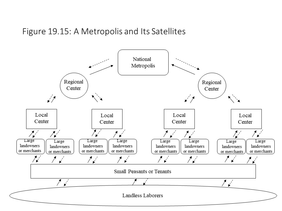
The world capitalist system consists of several national metropolises and each exercises its monopoly power. This position of power makes it possible for the metropolis to transfer surplus production to itself and away from the periphery through its control of pricing. The solid arrows and the dashed arrows in Figure 19.15 indicate that the flows traveling in an upward direction are larger than the flows traveling in the downward direction at each level. The differences between the upward flows and the downward flows represent the surplus.
The hierarchical structure depicted in Figure 19.15 does not exist within a competitive capitalist framework. That is, in competitive capitalism, workers confront capitalists but no complicated chain of metropolises and satellites will arise. The reason is that monopoly power is required for these networks to become established. Indeed, two kinds of monopoly give rise to these networks within the world capitalist economy.[61] The first kind is monopolistic merchant’s capital where merchants purchase products from local producers and then export them.[62] These merchant capitalists are not directly involved in production.[63] The second type is modern monopoly capital, which is based on large-scale capitalist production and modern production technology.[64]
Frank’s major point is that underdevelopment results from these interactions. Without investment in sectors that will promote the growth of employment and production in the satellites, the satellite nations will remain at a low level of development. Unfortunately for the periphery, it is the metropolis that decides how to use the large surpluses appropriated from the satellites and collected at the center. This situation poses long-term development problems for developing nations.
The development of capitalism on a global scale since the 1960s provides an abundance of evidence to test the theory. According to Felipe Antunes de Oliveira, “Frank’s prediction that no real development was possible within capitalism was almost immediately challenged by the facts.”[65] Economic growth in Latin America in the late 1960s and early 1970s and the rapid growth of East Asian countries in the 1980s and 1990s “seemed to provide further and conclusive evidence against Frank’s dependency theory.”[66] The burden then is on dependency theorists to explain these cases in a manner that is consistent with their overall approach to the world capitalist economy. Nevertheless, Antunes explains that the economic stagnation in the 1980s and more recent economic crises in Latin America imply that Frank’s theory “may still capture a deeper truth about the limits to peripheral development.”[67] Despite some challenging evidence, dependency theory provides us with a way of thinking about how aggregate surplus production is appropriated and redistributed throughout the world capitalist economy.
T he Theory of Unequal Exchange
One final alternative radical theory of world trade that we will consider is Arghiri Emmanuel’s theory of unequal exchange, which he developed in the early 1970s in his Unequal Exchange: A Study of the Imperialism of Trade (1972) . Emmanuel aimed to show that competitive interaction between rich and poor countries in the global marketplace could lead to a worsening terms of trade for poor countries. To obtain this result, Emmanuel built some key assumptions into his model. For example, he assumed that the world economy only consists of two nations. He also assumed that the profit rates in the rich and poor nations would equalize as a result of the free flow of global capital. If the profit rate of one nation exceeds the profit rate of another nation, then capital will flow to the nation with the highest profit rate, driving that profit rate down and pushing the other nation’s profit rate up until equalization occurs.
At the same time, Emmanuel assumes that wage rates in the rich and poor nations differ significantly because labor is not mobile. As Itoh explains, capital is relatively mobile, but labor is relatively immobile in Emmanuel’s framework due to immigration restrictions.[68] Howard and King also state that Emmanuel’s theory assumes “a powerful tendency for the rate of profit to be equalized on a world scale, while there remain huge differences in both wage rates and rates of exploitation between advanced and backward countries.”[69] As Emmanuel explains, he treats wages as the independent variable in his theoretical system.[70] Furthermore, he assumes that the rates of surplus value are “institutionally different” and not subject to competitive factor market equalization.[71] The fact that differences in rates of surplus value exist alongside wage differentials should make sense. If two nations have similar working day lengths but one nation has much lower wages, then the nation with much lower wages should have a higher rate of surplus value, other factors the same.
The persistent wage differentials are explained in terms of the immobility of labor, but what about the absolute levels of wages in the two nations? Emmanuel’s assumption about differential wages stems from Marx’s claim that the value of labor-power contains an “historical and moral element.”[72] The reader should recall that the value of labor-power depends on cultural and social factors that are specific to time and place. What constitutes a required bundle of commodities in a rich nation will be very different from the required bundle of commodities in a poor nation. Generally, the workers in a rich nation will be accustomed to having more and better quality commodities available to them than workers in poor nations. Hence, the value of labor-power and the wage rate will be higher in the rich nation and lower in the poor nation.
One might suspect that the wage differentials will lead to different prices across nations for the same product. This result does not necessarily follow though. For example, Emmanuel considered the possibility that two capitalist nations produce the same commodities but that one nation has a higher wage level.[73] For a common rate of profit and for a single production price to emerge, the higher wage nation must have higher productivity so that its other costs are lower and its overall costs are the same across the two nations.[74] The situation is easier to visualize by considering the diagram in Figure 19.16.
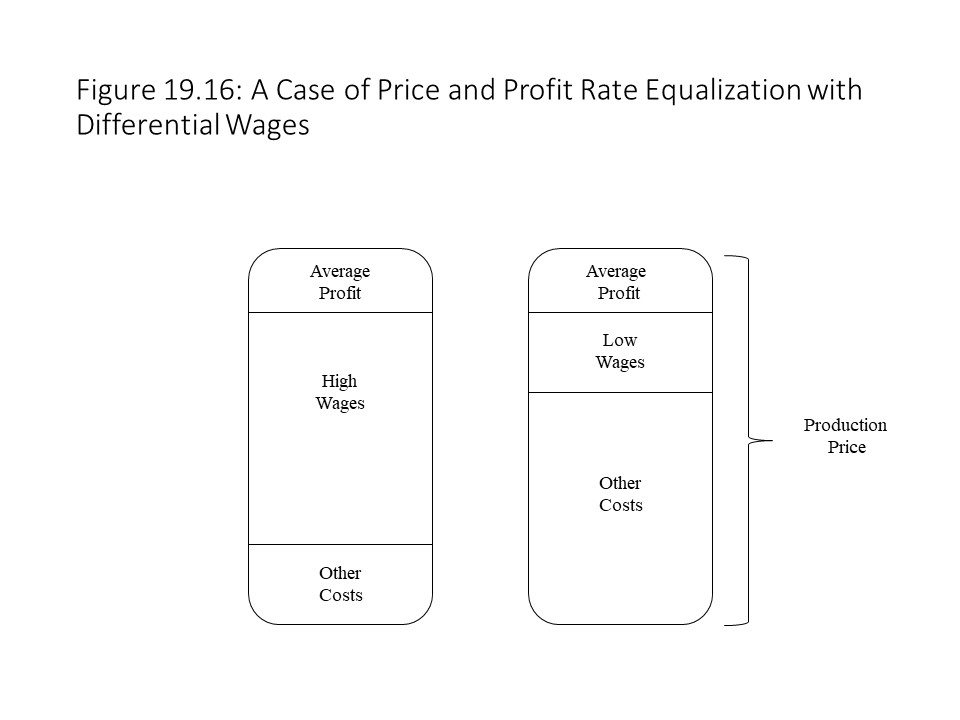 As Figure 19.16 shows, the higher wage nation has other production costs that are lower, which makes it possible for costs to be equal across the two nations. Indeed, the higher productivity is the cause of the higher wages. When adding the average profit to the equal costs, the production prices are the same. We thus see one example of how profit rates and production prices can be the same even when wages vary across nations.
We next consider an example in which two nations produce different commodities. As we learned in Chapter 8, Marx transformed values into production prices to explain how a general rate of profit is formed in the economy. Setting aside the criticism of Marx’s procedure, which has given rise to the Transformation Problem debate, we follow Emmanuel in using Marx’s procedure to equalize the rate of profit throughout the world economy. Let’s consider only two countries: the United States and Mexico. Consistent with Emmanuel’s approach, we will assume that one nation, in this case the United States, pays a higher wage to workers than the other nation (Mexico). Howard and King use a simple numerical example involving the same organic compositions of capital in two nations with one nation having a lower wage rate and a higher rate of surplus value.[75] Here we consider a similar example using basic algebra to illustrate the main findings of the theory.
For notational purposes, the high-wage United States will labeled nation A, and low-wage Mexico will be labeled nation B. The two nations produce different goods, but the organic composition of capital is the same in the two nations. The equal organic compositions of capital may be represented as follows:
In this equation, C and V refer to the constant capital and the variable capital in each nation. It is also assumed that wages are lower in Mexico, and the rate of surplus value is correspondingly higher in Mexico. These conditions are represented as follows:
In this inequality, S refers to the surplus value in each nation. We can now write the total value produced in each nation as the product of the physical quantity produced (q) in that nation and the value per unit (w) in that nation. The following equations thus hold:
The reader should recall that to obtain the rate of profit, we need to add the entire surplus value (S) in both nations and divide by the aggregate capital (C+V). Without subscripts, these aggregates refer to the combined sums for the two nations. That is,
The total production price (qp) in each nation may now be computed as the product of the output (q) in that nation and the per unit production price (p) in that nation. The total production price in each nation is then equal to the sum of the capital advanced and the average profit in that nation as follows:
Using this information, we can calculate the value ratio and the production price ratio. The value ratio is the ratio of the individual unit values (based on embodied labor) in the two nations. The price ratio is the ratio of the per unit production prices in the two nations. The ratios are calculated as follows:
Value ratio:
Production price ratio:
To give these equations meaning, suppose that we have the following information for the U.S. and Mexico:
| Nation | Constant Capital | Variable Capital | Surplus Value | Quantity Qroduced (q) |
| United States (A) | 600 | 300 | 200 | 130 |
| Mexico (B) | 300 | 150 | 300 | 110 |
| Aggregate | 900 | 450 | 500 |
It should be clear that the organic compositions of capital are the same in the two nations (C/V = 2). It should also be clear that the rate of surplus value (S/V) is higher in Mexico where wages (V) are lower. Using our equations to calculate the value ratio, the rate of profit, and the production price ratio, we obtain the following:
Value ratio:
Rate of profit:
Production price ratio:
The example shows that the production price ratio exceeds the value ratio. The implication is that the price of the commodity in the United States is relatively higher than what it should be given its relative value. Another way of stating the same result is to say that international competition causes the price of commodity A to be 1.69 units of commodity B. At the same time, if the commodities exchanged according to their values (i.e., labor content), then the price of commodity A would be 1.24 units of commodity B. The price of the U.S. commodity is thus higher than it would otherwise be. As Howard and King explain, the unequal exchange of commodities that results causes a transfer of value to the rich country, which worsens global inequality over time.[76] As the reader might recall, Marx showed how capitalist societies produce surplus value even when commodities exchange according to their values. He did acknowledge, however, that unequal exchanges can lead to the redistribution of value with one side to the exchange gaining and the other side losing. Emmanuel has shown how nations can be involved in such unequal exchanges leading to systematic value transfers from poor nations to rich nations.
A general claim may thus be stated and proven: If the production price ratio (pA/pB) exceeds the value ratio and two nations organic compositions of capital are the same, then the rate of surplus value must be higher in nation B. To prove this result, we proceed as follows:
With a bit of algebraic manipulation, this equation may then be rewritten as follows:
Because the organic compositions of capital are the same in the two nations, we can substitute CA/VA for CB/VB to obtain the following result:
With some additional algebraic manipulation, this equation may then be reduced to obtain the final result:
Therefore, the rate of surplus value in Mexico must exceed the rate of surplus value in the United States given these assumptions.
Emmanuel’s finding that rich nations benefit at the expense of poor nations is interesting because it is achieved without any reference to monopoly power or military intervention.[77] As Shaikh argues, Emmanuel demonstrated that “it is not necessary to abandon the law of competition in order to be able to understand the intrinsic determinants of modern imperialism.”[78] The result is obtained by means of an analysis of competitive interaction in the marketplace. It thus provides us with a way of thinking about how voluntary exchange in the international sphere can lead to a situation of worsening inequality between nations. Overall, international trade and the export of capital can be combined to explain how developing nations are exploited in the neocolonial era.[79]
Fo llowing the Economic News [80]
In a recent article in The Economic Times, Arvind Panagariya argues in favor of economics policies that will bring about a boom in exports in India. Panagariya claims that rapid economic growth in India will require a much greater presence in global markets. He explains that the Indian share of global merchandise exports is very low at only 1.7%. To achieve a greater influence in the international marketplace, Panagariya encourages the elimination of three strategies that have been a focus of Indian trade policy in the past. One strategy to eliminate is import substitution, which is a policy aimed at promoting the domestic production of products that will serve as substitutes for imported products. He also favors less promotion of small enterprises and a weaker rupee in the foreign exchange market. Panagariya does not believe that the import substitution strategy will succeed, but even if it does succeed, the elimination of import substitution as a strategy also makes sense when considered through the lens of new trade theory. If India succeeds at increasing exports of goods in industries that are likely to become retainable industries and then proceeds to capture even more retainable industries through an import substitution strategy, then it risks capturing so many retainable industries from other nations that its GDP and other nations’ GDPs begin to decline. This possibility involves India moving into the zone of mutual gain, where India can reduce the percentage of retainable industries it captures to the benefit of its trade partners and itself. As Panagariya argues, policies aimed at rapidly expanding exports should be joined with support for the rapid expansion of imports. Panagariya points to the rapid expansion of exports during the 2000s as an example. He explains that without the rapid expansion of exports, India could not have imported so many cell phones, which would have undermined the cell phone revolution in India. Therefore, India should aim to capture some retainable industries but an aggressive approach that does not allow its trade partners to capture some retainable industries will hurt India and its trade partners. Similarly, the emphasis on “micro and small enterprises” is a policy that Panagariya believes should be discarded. The capture of retainable industries depends upon growth in industries in which large economies of scale exist. An emphasis on small-scale production will make it impossible to reduce per unit production costs below those of competitors. The capture of retainable industries then becomes impossible. Finally, Panagariya advocates “a realistic exchange rate.” In other words, a weaker rupee will allow producers of exports to compete more effectively in international markets where their goods are cheaper as a result. The enhanced competitiveness that follows will make it possible for India to capture additional retainable industries. The trick is to capture many retainable industries but without overreaching to the detriment of India and its trading partners.
Summary of Key Points
- According to neoclassical economists, even if a nation has an absolute advantage in the production of two commodities, it may still benefit from trade if another country has a comparative advantage.
- When resources are heterogeneous, a nation experiences increasing marginal opportunity costs, but when resources are homogeneous, a nation experiences constant marginal opportunity costs.
- In the case of trade between two nations, the limits to the international terms of trade are the domestic terms of trade in each nation.
- When two nations specialize in the commodities in which they have comparative advantages, each can consume output combinations along a trading possibilities frontier that lies beyond the production possibilities frontier.
- In the case of increasing marginal opportunity costs, each nation will only pursue partial specialization because eventually the marginal opportunity costs become equal.
- The equilibrium terms of trade in the case of increasing marginal opportunity costs is given by the slope of the ray from the origin that passes through the intersection of the two nations’ offer curves.
- The basis of Ian Fletcher’s critique of comparative advantage is the existence of eight hidden assumptions that form the basis of the theory.
- Retainable industries are industries in which economies of scale are so large that the first nation to reach a large production volume captures and retains the industry.
- New trade theory suggests that free trade leads to a positive sum game of mutual gains at times and to a zero-sum game of bitter conflict at other times.
- According to neoclassical economists, import tariffs and import quotas lead to losses of social welfare because higher prices reduce the quantity demanded of consumers and increase the production of inefficient domestic producers.
- According to dependency theorists, a national metropolis appropriates the surpluses of multiple satellites by using its considerable market power.
- In the theory of unequal exchange, unequal exchanges in the international marketplace allow a high-wage nation to appropriate excess value from a low-wage nation when both nations possess the same organic compositions of capital and a higher rate of surplus value exists in the low-wage nation.
List of Key Terms
Comparative advantage
Absolute advantage
Increasing marginal opportunity costs
Heterogeneous resources
Homogeneous resources
Domestic terms of trade
International terms of trade
Limits to the terms of trade
Trading possibilities frontier (TPF)
Autarky
Partial specialization
Offer curves
Free trade
Kaldor-Hicks criterion
Retainable industries
Lockout phenomenon
Positive sum game
Zero-sum game
Rational protectionism
Import tariff
Import quota
Dependency theory
Underdevelopment
Center
Periphery
Metropolises
Satellites
Lumpenbourgeoisie
Monopolistic merchant’s capital
Modern monopoly capital
Unequal exchange
Value ratio
Production price ratio
Problems for Review
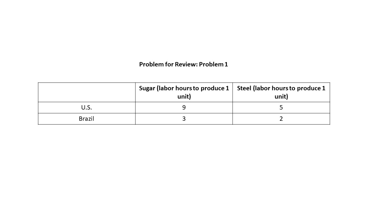
1. Given the information in the table below, determine which nation has an absolute advantage in the production of each commodity and which nation has a comparative advantage in the production of each commodity.
2. Given the information in Figure 19.17, answer the following questions:
- Which nation has an absolute advantage in sugar production?
- Which nation has an absolute advantage in steel production?
- Which nation has a comparative advantage in sugar production?
- Which nation has a comparative advantage in steel production?
- What are the limits to the international terms of trade? That is, what is the maximum and minimum price of sugar in terms of steel? What is the maximum and minimum price of steel in terms of sugar?
- If the international terms of trade are 1 unit of sugar/1 unit of steel, then add the new trading possibilities frontiers to the graphs for each nation. Label the intercepts.
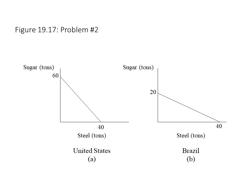 3. Given the information in Figure 19.18, answer the following questions:
- If a tariff of $0.60 is imposed as implied in the graph, then calculate the deadweight loss that results from the excess production costs of domestic producers. Hint: Recall the formula for the area of a triangle.
- Calculate the deadweight loss resulting from the reduction in quantity demanded.
- Calculate the tariff revenue.
- If an import quota of 70 units was imposed instead in this case, then which parties might acquire the windfall profit? Why?
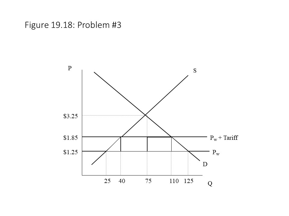 4. Suppose the two nations represented in the table below produce different commodities and trade in the international marketplace. Complete the table, and calculate the general rate of profit (r). Then calculate the value ratio and the production price ratio. How do these ratios compare? What role do the assumptions of this model play in producing this result?
| Nation | Constant Capital | Variable Capital | Surplus Value | Quantity Produced (q) |
| Nation A | 250 | 275 | 135 | 125 |
| Nation B | 200 | 220 | 75 | 110 |
| Aggregate |
- See Hunt (2002), p. 191-192, for a summary of Mill’s theory of international prices. ↵
- See Fletcher (2009), p. 105-118. ↵
- I am deeply grateful to Ian Fletcher for granting me permission to include this summary of his perspective. The original source is: Fletcher, Ian. Free Trade Doesn't Work: Why American Needs a Tariff. U.S. Business & Industry Council: Washington, DC, 2009. p. 105-118 and 215-231. Information about the most recent edition of his book may be found at: http://www.freetradedoesntwork.com/index.html↵
- Ibid. p. 105-106. ↵
- Ibid. p. 105. ↵
- Ibid. p. 105. ↵
- Ibid. p. 105. ↵
- Ibid. p. 106. ↵
- Ibid. p. 106-107. ↵
- Ibid. p. 107-109. ↵
- I rephrased this hidden assumption. Fletcher (2009), p. 109-110, states it somewhat differently. ↵
- Ibid. p. 110-113. ↵
- Ibid. p. 113-115. ↵
- Ibid. p. 114. ↵
- Ibid. p. 114. ↵
- Ibid. p. 115. ↵
- Noam Chomsky offers a similar critique of Ricardo’s original example involving England and Portugal in Chomsky (2002), p. 254. ↵
- Fletcher (2009), p. 115-118. ↵
- Ibid. p. 116. ↵
- Ibid. p. 116. ↵
- Ibid. p. 215. ↵
- Ibid. p. 215. ↵
- Ibid. p. 215. ↵
- Ibid. p. 216. ↵
- Ibid. p. 216. ↵
- Ibid. p. 216. ↵
- Carbaugh (2011), p. 88, makes the same point using a single, similarly shaped AC curve for two different nations. Although the firms have the same AC curves, the firm that produces the larger volume first ends up with a lower AC. ↵
- Fletcher (2009), p. 217. ↵
- Ibid. p. 220. ↵
- Ibid. p. 221. ↵
- Ibid. p. 221. ↵
- Ibid. p. 222. ↵
- Ibid. p. 222. ↵
- This graph is a modified version of the one that Fletcher (2009), p. 221, provides. A similar graph can be found in Gomory and Baumol (2000), p. 31. ↵
- Ibid. p. 224. ↵
- This graph is a modified version of the one that Fletcher (2009), p. 224, provides. A similar graph can be found in Gomory and Baumol (2000), p. 37. ↵
- Ibid. p. 223. ↵
- Ibid. p. 223-225. ↵
- Ibid. p. 228. ↵
- Ibid. p. 228. ↵
- Ibid. p. 229. ↵
- Ibid. p. 229. ↵
- Ibid. p. 229. ↵
- Ibid. p. 229. ↵
- Ibid. p. 229. ↵
- Ibid. p. 230-231. ↵
- Carbaugh (2011), p. 158. ↵
- Ibid. p. 158. ↵
- Ibid. p. 158. ↵
- Rose (2016). ↵
- Rose (2016) provides a simple diagram to demonstrate these relationships. ↵
- Frank (1969), p. 3. ↵
- Howard and King (1992), p. 177. ↵
- Frank (1969), p. 7. ↵
- Brewer (1992), p. 164. ↵
- Ibid. p. 196. ↵
- Ibid. p. 164. ↵
- Howard and King (1992), p. 177. ↵
- Howard and King (1992), p. 177. ↵
- Frank (1969), p. 7. ↵
- Brewer (1990), p. 166. ↵
- Ibid. p. 166. ↵
- Ibid. p. 166. ↵
- Ibid. p. 166. ↵
- Antunes (2017) ↵
- Antunes (2017) ↵
- Antunes (2017) ↵
- Itoh (2009), p. 207. ↵
- Howard and King (1992), p. 189. ↵
- Emmanuel (1972), p. 64. ↵
- Ibid. p. 64. ↵
- Brewer (1990), p. 209. ↵
- Brewer (1990), p. 203. ↵
- Ibid. p. 203. ↵
- Howard and King (1992), p. 190-191. ↵
- Howard and King (1992), p. 191. ↵
- Brewer (1990), p. 200. ↵
- Shaikh (1980), p. 210. ↵
- Itoh (2009), p. 207. ↵
- Panagariya, Arvind. “View: How to make exports boom [Foreign-Trade]. The Economic Times; New Delhi. 27 June 2019. ↵