Develop the fundamentals of balance of payments accounting
Explain how to work with foreign exchange rates
Analyze the determination of equilibrium exchange rates using supply and demand
Investigate the Theory of Purchasing Power Parity
Distinguish between fixed and floating exchange rate regimes
Explore Marxist theories of imperialist finance and exchange rate determination
This final chapter of the book considers theories of international finance. As the reader may have noticed, not much was said about the role of money in the previous chapter. Curiously, neoclassical economists have a tradition of separating the field of international economics into these two parts. Part of this chapter concentrates on the accounting method, referred to as balance of payments accounting, which is used to describe the financial flows between one nation and the rest of the world. The neoclassical model of supply and demand, as applied to the foreign exchange market or currency market, is also developed in this chapter to explain how exchange rates are determined in competitive markets. Using this framework, we will explore the role of exchange rate adjustments in equalizing purchasing power across nations. We will also consider the role of the central bank in foreign exchange markets and see why currency crises sometimes occur. Finally, we will examine Marxist theories of imperialist finance to provide us with an alternative perspective on the same topic.
Balance of Payments Accounting
When a nation interacts with the rest of the world, it engages in a wide variety of transactions. A nation buys and sells goods and services in international commodity markets. It receives interest payments and pays interest in international financial markets. Domestic employers in that nation also pay foreign employees just as foreign employers sometimes pay domestic employees. Public and private transfer payments are often made from a nation to other nations, or such transfers are received by a nation. Investors in a nation also often buy financial assets like stocks and bonds or the investors sell them to other nations. Economists find it necessary to have a way of recording all these transactions so that they can study how these interactions influence the overall health and direction of a nation’s economy.
Balance of payments accounting refers to the method of accounting for all international transactions that occur between one nation and the rest of the world. Its counterpart at the domestic level is national income accounting, which we thoroughly analyzed in Chapter 12. The method involves recording each transaction between a nation and the rest of the world as a debit or a credit, depending on the nature of the transaction. For example, a transaction that leads to a payment to the United States from another nation is recorded as a credit in the U.S. Balance of Payments and is thus given a positive value. Any transaction that leads to a payment from the United States to another nation is recorded as a debit in the U.S. Balance of Payments and is thus given a negative value.
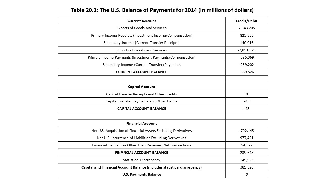
Table 20.1 shows a summary of the U.S. Balance of Payments for 2014.
It is helpful to think about which types of transactions lead to credits or debits in the U.S. Balance of Payments. For example, when the U.S. exports goods and services, these transactions are recorded as credits because these sales lead to payments to U.S. sellers. When an American investor receives an interest payment from a foreign borrower, the transaction is recorded as a credit as well. When an American worker receives compensation for work performed by a foreign firm, the payment is recorded as a credit. If an American family receives private transfer payments (referred to as remittances) from a family member working in another nation, the transfer payment is recorded as a credit. Each of these transactions is recorded in a subaccount of the Balance of Payments referred to as the current account. The current account only includes transactions that do not involve the purchase or sale of an income-earning asset.
Just as credits may be recorded in the current account, debits may also be recorded. For example, when the U.S. imports goods and services, these transactions are recorded as debits in the U.S. current account because these purchases lead to payments from U.S. buyers to foreign sellers. If an American borrower makes an interest payment to a foreign lender, then the payment is recorded as a debit in the current account. If a U.S. employer pays a salary to a foreign worker, then the payment is treated as a debit in the current account. If the U.S. government grants monetary aid to a foreign nation, then the public transfer payment is treated as a debit in the U.S. current account. Once all the credits and debits are added up in the U.S. Current Account, the final calculation is referred to as the Current Account Balance. When this figure is positive, it is said that a current account surplus exists. When this figure is negative, it is said that a currentaccount deficit exists. Table 20.1 shows that a current account deficit of over $389.5 billion existed in 2014.
One subaccount of the Balance of Payments is worth mentioning because it is frequently cited in the financial news. The trade balance, as it is commonly known, refers to the difference between exports of goods and services and imports of goods and services. In this case, imports exceed exports of goods and services by about $508 billion. Therefore, a negative U.S. trade balance of approximately $508 billion existed in 2014. When a negative trade balance exists, it is referred to as a trade deficit. If exports exceed imports of goods and services, then a positive trade balance exists, which is referred to as a trade surplus. If the balance happens to be exactly zero, which would be extremely unlikely in practice, then balanced trade exists.
In addition to the current account, another important subaccount is called the capital account. Transactions that are recorded in the capital account involve the purchase and sale of nonfinancial assets like copyrights, patents, and trademarks. When these transactions involve sales of nonfinancial assets, they are recorded as credits. When they involve purchases of nonfinancial assets, they are recorded as debits. For example, if a copyright owned by an American firm is sold to a Chinese firm, then the payment received by the American firm is recorded as a credit in the U.S. Capital Account. If a patent owned by a German firm is sold to an American firm, then the payment made by the American firm is recorded as a debit in the U.S. Capital Account.
The final subaccount of interest is the financial account. Transactions that are recorded in the financial account involve the purchase and sale of financial assets like stocks and bonds. Examples include purchases and sales of corporate and government bonds, foreign direct investment, and central bank purchases and sales of securities. When these transactions involve sales of financial assets, they are recorded as credits. When they involve purchases of financial assets, they are recorded as debits. For example, if an American bondholder sells a U.S. government bond to a foreign investor, then the payment that the bondholder receives is recorded as a credit in the U.S. Financial Account. If a foreign investor purchases newly issued shares of stock in an American company, then the transaction is recorded as a credit in the financial account because an American firm receives a payment. If the U.S. Federal Reserve sells securities to the Bank of Japan in exchange for Japanese yen, then the transaction is recorded as a credit in the U.S. Financial Account. In the last case, official reserve holdings increase. Official reserves include items like foreign currencies and gold held by a nation’s central bank.
On the other hand, if an American investor buys a bond from a foreign bondholder, then the payment to the foreign bondholder is recorded as a debit in the U.S. Financial Account. Similarly, if an American investor purchases a controlling stake in a foreign corporation, the payment to the corporation for the shares is recorded as a debit in the U.S. Financial Account. Finally, if the Bank of England sells U.S. Treasury bonds to the U.S. Federal Reserve, then the payment that the Fed makes to the Bank of England is recorded as a debit in the U.S. Financial Account. If the Fed makes the purchase using British pounds, then U.S. official reserves fall by an equal amount. Overall, if the credits in the capital account and financial account exceed the debits in the capital account and financial account, then a capital and financial account surplus exists. On the other hand, if the debits in the capital account and financial account exceed the credits in the capital account and financial account, then a capital and financial account deficit exists.
We are now in a much stronger position to understand the information presented in Table 20.1. The table shows that a current account deficit existed in the U.S. in 2014. Similarly, the table reveals that a capital and financial account surplus also existed in the U.S. in 2014. In theory, the current account and the capital and financial account should always add up to zero. That is, the overall U.S. Balance of Payments should be balanced with neither a surplus nor a deficit. The reason is that balance of payments accounting uses a double entry bookkeeping method. For every credit that is entered, a corresponding debit must be entered. Similarly, for every debit that is entered, a corresponding credit must be entered. For example, suppose that a U.S. company sells computers to a firm in France. As we have seen, exports are recorded as credits in the balance of payments because a payment is received for the exported goods. What is the offsetting debit in the U.S. Balance of Payments? Suppose that the French company pays for the computers with Euros. The America firm will then deposit the Euros in a Euro-denominated bank account in, let’s say, France. This transaction requires a payment to the French bank in exchange for that financial asset (i.e., the bank deposit). Therefore, the transaction is recorded as a debit in the financial account in an amount that exactly offsets the credit associated with the exports in the current account. All transactions that occur between the home nation and the rest of the world can be analyzed in the same manner. As a result, all debits and credits should cancel out in the aggregate, even though each subaccount may show a surplus or deficit.
This result can be proven as follows. Suppose that we add up all the credits in the current account and all the credits in the capital and financial account. Now suppose that we add up all the debits in the current account and all the debits in the capital and financial account. Given what has been said about every credit having a corresponding debit and vice versa, it must be true that the sum of all credits equals the sum of all debits. If CA refers to the current account, KA+FA refers to the capital and financial account, and the subscripts refer to credits (c) and debits (d) in that specific subaccount, then the following must hold:
Rearranging the terms in the above equation yields the following result:
In other words, a current account surplus (an excess of credits over debits in the current account) necessarily implies a capital and financial account deficit (an excess of debits over credits in the capital and financial account). Similarly, a current account deficit (debits > credits in the current account) necessarily implies a capital and financial account surplus (credits > debits in the capital and financial account).
Although the balance of payments cannot show a surplus or deficit overall, in practice, statisticians must estimate the total credits and debits in each subaccount. Because statistical estimates do not guarantee completely accurate results, the current account balance is never exactly offset by the capital and financial account balance. Therefore, the difference must be included, which is referred to as statistical discrepancy. Once we add this figure in Table 20.1, the surplus in the capital and financial account exactly offsets the current account deficit.
The Net International Investment Position
The balance of payments is a record of all international flows of goods and services, interest payments, transfers, and financial and non-financial assets between one nation and the rest of the world. Because the items on the statement are all flows, they are measured during a given period, such as a year or a quarter. Economists are also interested in keeping a record of the stocks of all foreign financial assets and foreign financial liabilities that a nation possesses at any one time. The difference between a nation’s foreign financial assets and its foreign financial liabilities at a point in time is called its net investment position. The statement that contains this information is called the Net International Investment Position. It is a bit like a balance sheet for the entire nation, and the net investment position is somewhat like the net worth of the nation.
The U.S. Net International Investment Position for 2014 is shown in Table 20.2.
As Table 20.2 shows, the net international investment position for the U.S. in 2014 was a negative value exceeding $7 trillion. This amount was the net foreign debt of the United States in 2014. This figure means that U.S. liabilities with respect to the rest of the world exceeded U.S. ownership of foreign assets. The U.S. was considered a net debtor in 2014 because it owed more to the rest of the world than was owed to it. If its foreign-owned assets exceeded its foreign liabilities, then it would be regarded as a net creditor.
An interesting relationship exists between the Balance of Payments and the Net International Investment Position of a nation. Specifically, a nation that receives more from the rest of the world than it spends runs a current account surplus. Its corresponding capital and financial account deficit implies that it lends this amount to the rest of the world by purchasing foreign assets. The increase in its stock of foreign assets increases its net investment position and moves it in the direction of net creditor status.
Similarly, a nation that spends more than it receives from the rest of the world runs a current account deficit. Its corresponding capital and financial account surplus implies that it borrows this amount from the rest of the world by selling assets to foreign investors. The increase in its foreign liabilities worsens its net investment position and moves it in the direction of net debtor status. As a result, the current account deficit that the U.S. experienced in 2014 worsened the U.S. net international investment position by this amount. In other words, the current account deficit in 2014 increased America’s net foreign debt.
It is possible to use the national income accounts identity from Chapter 12 to show how a current account balance relates to a nation’s government budget and private sector gaps. The identity below shows how a nation’s GDP (Y) may be calculated as the sum of the different components of spending on final goods and services.
In the above identity, C refers to personal consumption expenditures, I refers to gross private domestic investment, G refers to government expenditures, and NX refers to expenditures on net exports (i.e., exports minus imports).
Subtracting taxes (T) and consumer spending (C) from both sides of the equation and substituting X – M for NX yields the following result.
The left-hand side of the equation represents total saving, which is equivalent to disposable income (Y-T) minus consumer spending. We can thus substitute saving (S) into the equation to obtain the following result.
Solving for the trade balance (i.e., net exports), we can write the equation as follows:
If we ignore primary and secondary income payments and receipts (i.e., investment payments, compensation, and transfers), then the nation’s trade balance is the same as the current account balance. Therefore, the current account balance equals the sum of the private sector gap and the government budget gap. For example, if a current account surplus exists, then the nation is a net lender for the year, strengthens its net international investment position, and may achieve this goal with positive net saving in the private sector (S > I) and a government budget surplus (T > G). Net saving in the private and public sectors thus corresponds to net lending in the world economy. On the other hand, if a current account deficit exists, then the nation is a net borrower for the year, worsens its net international investment position, and may bring about this result with negative net saving in the private sector (S < I) and a government budget deficit (T < G). Net borrowing in the private and public sectors thus corresponds to net borrowing in the world economy.
Working with Foreign Exchange Rates
Now that we have an accounting framework for thinking about a nation’s international transactions, we will shift gears and begin thinking about how foreign exchange markets work. Once we have a theory that helps us understand how these markets function, we will circle back and connect that theory to balance of payments accounting.
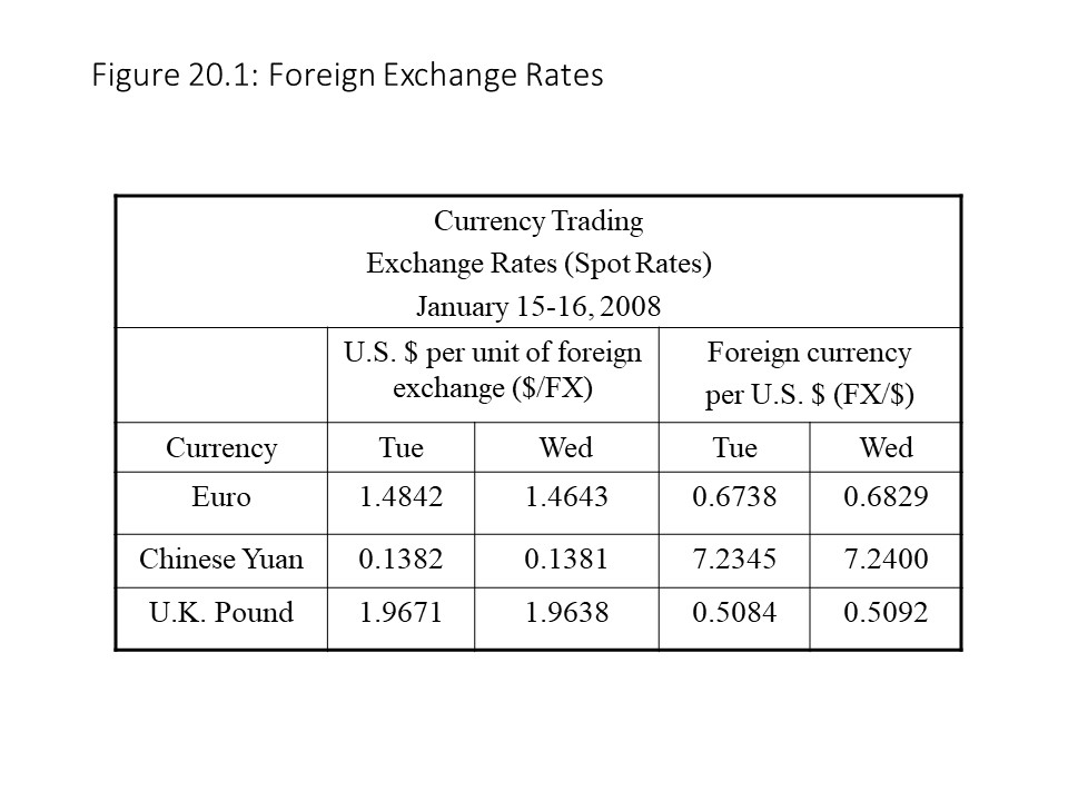
Before we explore the inner workings of foreign exchange markets, we need to consider what foreign exchange rates are and what they mean. On any given day, it is possible to turn to the financial news section of The Wall Street Journal and see the current exchange rates. For example, Figure 20.1 provides information about current spot rates (foreign exchange rates) for two consecutive days in January 2008.[3]
Foreign exchange rates simply tell us what the price of one nation’s currency is in terms of another nation’s currency. For example, on Tuesday, January 15, 2008, the price of one Euro was about $1.4842. By Wednesday, January 16, 2008, the price of a Euro was only $1.4643. The price of a Euro had thus fallen from one day to the next. The prices of the Chinese Yuan and the U.K. Pound had also fallen. The Yuan fell from $0.1382 to $0.1381, and the U.K. Pound fell from $1.9671 to $1.9638. All these currencies fell in value relative to the U.S. dollar over the course of these two days. When a currency’s value declines relative to another currency, we say that it has depreciated against the other currency.Figure 20.1, we see a rather different result. From Tuesday to Wednesday, each of these numbers increased. For example, the price of $1 on Tuesday, January 15, 2008 was 0.6738 Euros and on Wednesday it was 0.6829 Euros. That is, the dollar increased in value relative to the Euro. The situation was similar with the other two currencies. The U.S. dollar increased in value from 7.2345 to 7.2400 Yuan and from 0.5084 to 0.5092 pounds. Whenever a currency increases in value relative to another, we say that the currency has appreciated relative to the other currency.
It is no coincidence that each of these foreign currencies depreciated against the U.S. dollar while the U.S. dollar appreciated against them. In fact, it must be the case. The reader may have noticed that the calculations in the two columns on the left are in terms of U.S. dollars per unit of foreign exchange ($/FX) whereas the calculations in the two columns on the right are in terms of foreign exchange per U.S. dollar (FX/$). The one calculation is the reciprocal of the other. Therefore, if an increase occurs from one day to the next in the first two columns, then a decrease must occur from one day to the next in the final two columns, and vice versa.
For these exchange rates to change from one day to the next is not exceptional. In fact, foreign exchange rates typically change from minute to minute. Consider, for example, the U.S. dollar-U.K. pound exchange rate during the period from May 26 to July 2, 2015 shown in Figure 20.2.
The pound fluctuated during that short period from less than $1.52 to almost $1.59. Much larger fluctuations can sometimes occur, as we will discuss later in the chapter.
Explaining Foreign Exchange Rate Fluctuations
It is natural to wonder why these fluctuations of exchange rates occur. The answer is that exchange rates are determined competitively in international currency markets or foreign exchange markets. As buyers and sellers change their purchases and sales for a huge variety of reasons, the market prices of foreign currencies change in response. To explain market prices in Chapter 3, we used the supply and demand model. In this chapter, we will once again turn to the supply and demand model to understand how equilibrium exchange rates and equilibrium quantities exchanged are determined.
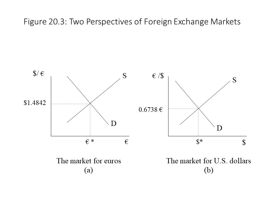
In the market for any currency, we can speak about the supply and demand for that currency. The sellers of the currency represent the supply side of the market, and the buyers of the currency represent the demand side of the market. Their competitive interaction determines the exchange rate and the amount exchanged. Figure 20.3 (a) offers an example of supply and demand in the market for Euros.
The equilibrium exchange rate of $1.4842 per Euro occurs where the quantity demanded and the quantity supplied of Euros are equal. If the exchange rate exceeds this level, then a surplus of foreign exchange will exist, and competition will drive the exchange rate down. If the exchange rate falls short of this level, then a shortage of foreign exchange will exist, and competition will drive the exchange rate up. The equilibrium quantity exchanged of Euros (€*) is also determined as competition brings about the equilibrium outcome in the market.Figure 20.3.
Also of importance is the relationship between the supply and demand curves in each market. The sellers supplying Euros in the Euro market must also be demanding U.S. dollars in the dollar market. Similarly, the buyers of Euros in the Euro market must also be supplying U.S. dollars in the dollar market. Think about an American who goes to Europe on vacation. She wants to buy some souvenirs but needs Euros to do so. She buys Euros and must sell U.S. dollars to do so. Similarly, a European tourist in the United States must sell Euros to buy U.S. dollars. To sell one is to buy the other and to buy one is to sell the other. In summary, the two markets are mirror reflections of one another.
The mirror reflection argument applied to foreign exchange markets is consistent with what we said earlier about the reciprocal relationship between the exchange rates. For example, suppose that the demand for Euros increases, shifting the demand curve for Euros to the right in Figure 20.4 (a).
The rightward shift of demand in the market for Euros corresponds to a rightward shift of supply in the market for U.S. dollars. As mentioned previously, buyers of Euros are sellers of U.S. dollars when we are discussing the dollar-euro and euro-dollar markets. The consequence is an appreciation of the Euro and a depreciation of the U.S. dollar, reflecting the reciprocal connection between these exchange rates. The equilibrium quantities exchanged of both Euros and U.S. dollars increase as well.
Building the Supply and Demand Model of Foreign Exchange Markets
It is easy to declare that supplies and demands for foreign currencies exist, but we really need to build the supply and demand model of foreign exchange markets from scratch to understand the underlying determinants of exchange rate movements. We will begin with the demand side of a foreign currency market. As stated previously, we can consider the market for foreign exchange or the market for the domestic currency (e.g., U.S. dollars) since each is just a mirror reflection of the other. Throughout the remainder of this chapter, we will adopt the perspective of a market for foreign exchange. The reason for doing so is that we are accustomed to thinking of products and services as having dollar prices. For example, the price of an automobile is stated in terms of dollars per automobile ($/auto). We can think of the price of Japanese Yen in the same way. That is, the price of the Yen (¥) is in terms of so many dollars per Yen ($/¥). If the exchange rate (e) rises, then the Yen appreciates, just as a rise in the price of an automobile would mean that it has appreciated in value. Whenever we consider exchange rates, therefore, we will refer to dollars per unit of foreign exchange ($/FX).
Figure 20.5 shows a downward sloping demand curve for foreign exchange.
As the exchange rate falls, the foreign currency becomes cheaper and the quantity demanded of foreign exchange rises. It is worth asking why the demand curve slopes downward in this case.[4] When we learned about product markets, it seemed obvious that a lower price for a good, like apples, would lead to a rise in the quantity demanded of apples, ceteris paribus. As the price falls, other things the same, consumers are willing and able to buy more apples. The problem is that the explanation does not seem quite so obvious in the case of a foreign currency. After all, we do not eat Euros and so a lower price may not seem like it would automatically lead to increased purchases. Although we do not eat foreign currencies, they are useful as a means to an end. That is, if we wish to buy foreign goods and services, then we need to buy foreign currencies. Therefore, when the price of a foreign currency declines, we buy more of it because it allows us to purchase more foreign goods and services. That is, foreign goods and services become cheaper when the exchange rate ($/FX) falls and so we purchase more of the foreign currency.
In addition to imported goods and services becoming cheaper when the exchange rate falls, it is also true that foreign assets become cheaper when the exchange rate falls. That is, foreign stocks, bonds, and businesses become less expensive and so investors buy more foreign currency when its price falls. In this case, foreign currency is viewed as a means to buy foreign assets.
A final reason why the demand curve for foreign exchange slopes downward deals with currency speculation. That is, when the price of a foreign currency falls, speculators may expect it to rise later to some normal level. Therefore, speculators will purchase more as the exchange rate falls because they will anticipate a capital gain from the later appreciation of the currency.[5]
These three factors combine to create a downward sloping demand for foreign exchange. We could easily reverse the logic for all three factors to explain what happens when the exchange rate rises. When the exchange rate rises, the foreign currency becomes more expensive. Therefore, imports of goods and services become more expensive as do foreign assets. Furthermore, speculators will expect the exchange rate to fall later and so they expect a capital loss in the future. As a result, speculators will buy less foreign exchange.
We have now explained movements along the downward sloping demand curve for foreign exchange, but shifts of the demand curve for foreign exchange are possible too. Figure 20.6 shows a rightward shift of the demand curve for foreign exchange.
In Figure 20.6 a rise in the quantity demanded of foreign exchange occurs at every possible exchange rate. Which factors might cause such a shift of the demand curve for foreign exchange?[6] The first factor that we will consider is a change in consumers’ preferences in the home nation. For example, let’s suppose that American consumers develop a stronger preference for a specific nation’s automobiles. In that case, the demand for that foreign currency will increase. That is, the quantity demanded of the foreign currency will rise at every exchange rate, resulting in a rightward shift of the demand curve. If for some reason, the preferences of Americans changed such that they wanted fewer automobiles at each exchange rate, then the demand curve would shift to the left.
A second factor that might shift the demand curve for foreign exchange is a change in consumers’ incomes in the home nation. For example, suppose that Americans experience a rise in their incomes due to an economic expansion. They will demand more goods and services as well as more assets. This greater demand for goods, services, and assets, includes a greater demand for the goods, services, and assets of foreign nations. In this case, we would expect a higher demand for foreign exchange and a rightward shift of the demand curve for foreign exchange. On the other hand, if Americans experience a drop in their incomes due to a recession, then they will demand fewer goods, services, and assets, including the goods, services, and assets of other nations. As a result, the demand for foreign exchange will decline, and the demand curve for foreign exchange will shift to the left.
A third factor that might shift the demand curve for foreign exchange is a change in the relative price levels of the two nations. For example, suppose that the price level in the U.S. rises while the price level in the foreign nation remains the same. In that case, Americans will view foreign goods, services, and assets as relatively cheaper. Therefore, they will demand a great amount of foreign exchange to buy these relatively less expensive foreign commodities and assets. The same result would occur if the U.S. price level remained the same and the foreign price level fell. On the other hand, a drop in the U.S. price level and/or a rise in the foreign price level would lead to a reduction in the demand for foreign exchange because U.S. goods, services, and assets would now be relatively cheaper than foreign commodities and assets.
A fourth factor that might shift the demand curve for foreign exchange is a change in the relative interest rates of the two nations. For example, suppose that interest rates in the foreign nation rise while interest rates in the U.S. remain the same. American investors will view foreign assets as better investments because they now pay more interest. The reader should also recall that as foreign interest rates rise, foreign asset prices will fall. Therefore, foreign assets will be viewed as a bargain and the demand for foreign exchange will increase. As a result, the demand curve for foreign exchange will shift to the right. The same result would occur if U.S. interest rates fell while foreign interest rates remained the same. American investors would view foreign interest-bearing assets as the better investments and would thus demand more foreign exchange. On the other hand, if U.S. interest rates rose as foreign interest rates remained the same or fell, then the demand for foreign exchange would fall and the demand curve for foreign exchange would shift to the left as American investors shied away from foreign investments.
A fifth and final reason that we will consider for shifts of the demand curve for foreign exchange deals with currency speculation. For example, suppose that the expectations of speculators change such that the exchange rate is expected to rise soon. In other words, they expect the foreign currency to appreciate soon. In that case, the demand for foreign exchange will rise as speculators decide to buy the currency before it appreciates. As a result, the demand curve for foreign exchange will shift to the right. Alternatively, suppose that speculators decide that the foreign currency is expected to depreciate soon. In that case, speculators will demand less foreign exchange, and the demand curve for foreign exchange will shift to the left. That is, speculators do not want to buy the foreign exchange because they expect it to lose value soon.
In these examples, it is important to keep in mind the distinction between a movement along the demand curve for foreign exchange and a shift of the demand curve. Movements along the demand curve for foreign exchange are caused by changes in the exchange rate. Shifts of the demand curve for foreign exchange, on the other hand, result from changes in any other factors that might affect the buyers of foreign exchange. This distinction is the same one discussed in Chapter 3 between a change in quantity demanded and a change in demand. Understanding the difference helps prevent possible confusions that might otherwise arise. For example, the reader may have noticed that speculative behavior has been used to explain both a movement along the demand curve and a shift of the demand curve for foreign exchange. In the case of a movement along the demand curve, the speculative response is a direct response to a falling exchange rate. In the case of a shift of the demand curve, speculators experience a change in their expectations that is not related to a change in the current exchange rate.
The situation is very similar on the supply side of the foreign exchange market. Indeed, the same factors should be at play on the supply side since the supply of foreign exchange is the mirror reflection of the demand for dollars. Because the demand for dollars is affected by the factors that we just described, the supply of foreign exchange must be affected by these same factors.
Figure 20.7 shows an upward sloping supply curve for foreign exchange.
As the exchange rate rises, the foreign currency becomes more expensive and the quantity supplied of foreign exchange rises. It is worth asking why the supply curve slopes upward in this case. When we learned about product markets, it seemed obvious that a higher price for a good, like apples, would lead to a rise in the quantity supplied of apples, ceteris paribus. As the price rises, other things the same, producers are willing and able to sell more apples. In the case of foreign exchange markets, sellers are willing and able to sell more foreign exchange because when they sell foreign exchange, they acquire U.S. dollars, which are useful as a means to an end. That is, if foreigners wish to buy American goods and services, then they need to buy U.S. dollars. Therefore, when the price of a foreign currency rises, they sell more of it because it allows them to purchase more American goods and services. That is, American goods and services become cheaper when the exchange rate ($/FX) rises and so they sell more of the foreign currency.
In addition to U.S. exports of goods and services becoming cheaper to foreign consumers when the exchange rate rises, it is also true that American assets become cheaper to foreign investors when the exchange rate rises. That is, American stocks, bonds, and businesses become less expensive and so foreign investors sell more foreign currency when its price rises. In this case, U.S. dollars are viewed as a means to buy American assets.
A final reason why the supply curve for foreign exchange slopes upward deals with currency speculation. That is, when the price of a foreign currency rises, speculators may expect it to fall later to some normal level. Therefore, speculators will sell more of the foreign currency as the exchange rate rises because they will anticipate a capital loss from the later depreciation of the currency if they do not sell now.
These three factors combine to create an upward sloping supply for foreign exchange. We could easily reverse the logic for all three factors to explain what happens when the exchange rate falls. When the exchange rate falls, the foreign currency becomes less expensive. Therefore, U.S. exports of goods and services become more expensive to foreigners as do foreign assets, and so less foreign exchange will be sold. Furthermore, speculators will expect the exchange rate to rise later and so they expect a capital gain in the future. As a result, speculators will decide to sell less foreign exchange.
We have now explained movements along the upward sloping supply curve for foreign exchange, but shifts of the supply curve for foreign exchange are possible too. Figure 20.8 shows a rightward shift of the supply curve for foreign exchange.
In Figure 20.8 a rise in the quantity supplied of foreign exchange occurs at every possible exchange rate. Which factors might cause such a shift of the supply curve for foreign exchange? Just as in the case of the demand for foreign exchange, it is possible that consumer preferences in the foreign nation change. For example, let’s suppose that foreign consumers develop a stronger preference for American automobiles. In that case, the supply of the foreign currency will increase. That is, the quantity supplied of the foreign currency will rise at every exchange rate, resulting in a rightward shift of the supply curve. If for some reason, the preferences of foreigners changed such that they wanted fewer American automobiles at each exchange rate, then the supply curve would shift to the left.
A second factor that might shift the supply curve for foreign exchange is a change in consumers’ incomes in the foreign nation. For example, suppose that foreigners experience a rise in their incomes due to an economic expansion. They will demand more goods and services as well as more assets. This greater demand for goods, services, and assets, includes a greater demand for the goods, services, and assets of the United States. In this case, we would expect a higher supply of foreign exchange and a rightward shift of the supply curve for foreign exchange. On the other hand, if foreigners experience a drop in their incomes due to a recession, then they will demand fewer goods, services, and assets, including the goods, services, and assets of the United States. As a result, the supply of foreign exchange will decline and the supply curve for foreign exchange will shift to the left.
A third factor that might shift the supply curve for foreign exchange is a change in the relative price levels of the two nations. For example, suppose that the price level in the foreign nation rises while the price level in the U.S. remains the same. In that case, foreigners will view U.S. goods, services, and assets as relatively cheaper. Therefore, they will sell a greater amount of foreign exchange to obtain dollars with which they can buy these relatively less expensive American commodities and assets. The same result would occur if the foreign price level remained the same and the American price level fell. On the other hand, a drop in the foreign price level and/or a rise in the American price level would lead to a reduction in the supply of foreign exchange because foreign goods, services, and assets would now be relatively cheaper than American commodities and assets.
A fourth factor that might shift the supply curve for foreign exchange is a change in the relative interest rates of the two nations. For example, suppose that interest rates in the United States rise while interest rates in the foreign nation remain the same. Foreign investors will view U.S. assets as better investments because they now pay more interest. Furthermore, if U.S. interest rates rise, U.S. asset prices will fall. Therefore, U.S. assets will be viewed as a bargain and the supply of foreign exchange will increase. As a result, the supply curve for foreign exchange will shift to the right. The same result would occur if foreign interest rates fell while U.S. interest rates remained the same. Foreign investors would view American interest-bearing assets as the better investments and would thus supply more foreign exchange. On the other hand, if foreign interest rates rose as U.S. interest rates remained the same or fell, then the supply of foreign exchange would fall and the supply curve for foreign exchange would shift to the left as foreign investors shied away from American investments.
A fifth and final reason that we will consider for shifts of the supply curve for foreign exchange deals with currency speculation. For example, suppose that the expectations of speculators change such that the exchange rate is expected to fall soon. In other words, they expect the foreign currency to depreciate soon. In that case, the supply of foreign exchange will rise as speculators decide to sell the currency and avoid potential losses from its future depreciation. As a result, the supply curve for foreign exchange will shift to the right. Alternatively, suppose that speculators decide that the foreign currency is expected to appreciate soon. In that case, speculators will supply less foreign exchange, and the supply curve for foreign exchange will shift to the left. That is, speculators will not want to sell the foreign currency because they expect it to gain value soon.
Once again, the distinction between a movement along the supply curve and a shift of the supply curve is important to keep in mind. Movements along the supply curve are always caused by changes in the exchange rate. Shifts of the supply curve, on the other hand, are always caused by changes in any other factors that influence sellers of foreign exchange aside from exchange rate changes. This distinction is the same one discussed in Chapter 3 between a change in quantity supplied and a change in supply.
We are now able to combine the supply and demand sides of the foreign exchange market to provide a more thorough explanation of the equilibrium exchange rate and the equilibrium quantity exchanged of foreign exchange. Furthermore, we use the model to explain how exchange rates change in response to exogenous shocks. That is, using the method of comparative statics, we can analyze how changes in consumers’ preferences, consumers’ incomes, relative price levels, relative interest rates, and the expectations of speculators can cause the equilibrium exchange rate and the equilibrium quantity exchanged to change in a specific foreign exchange market.
For example, suppose that American consumers learn about a new European automobile that is spacious, comfortable, and environmentally friendly. The popularity of this product causes American consumers to increase their demand for Euros so that they can purchase these automobiles. The demand for Euros will shift to the right as shown in Figure 20.9 (a).
The higher demand for Euros creates a shortage or an excess demand for Euros. As a result, competition drives up the exchange rate and the quantity exchanged of the Euro to their new equilibrium values of e2 and Q2. In this case, the Euro appreciates relative to the dollar.
Consider a different example. Suppose that interest rates in Japan fall significantly relative to interest rates in the United States. American investors will find Japanese assets to be less attractive investments, and they will want to purchase fewer of them. As a result, they will demand fewer Yen. The demand for Yen will shift to the left as shown in Figure 20.9 (b). The lower demand for Yen creates a surplus or an excess supply of Yen. Competition then drives the exchange rate and the quantity exchanged of Yen down to their new equilibrium values of e2 and Q2. In this case, the Yen depreciates relative to the dollar.
As another example, consider what will happen if speculators conclude that the Mexican peso will depreciate soon. They will want to sell pesos quickly before they lose value, and the supply of pesos will rise in the foreign exchange market. As a result, the supply curve shifts to the right, as shown in Figure 20.10 (a).
The resulting surplus or excess supply of pesos puts downward pressure on the peso. The exchange rate falls and the quantity exchanged of pesos rises to their new equilibrium values of e2 and Q2. In this case, the peso has depreciated. The belief that the peso will depreciate turns out to be accurate, but it is also a self-fulfilling prophecy. That is, speculators’ belief that the peso will soon depreciate brings about its depreciation. Such self-fulfilling prophecies are not unusual in foreign currency markets and can often create considerable volatility.
Finally, let’s consider a case where the price level in the United States rises relative to the price level in Britain. In this case, British consumers will find American exports of goods and services to be more expensive. As a result, they will demand fewer American exports and so they will supply fewer pounds in the foreign exchange market, as shown in Figure 20.10 (b). The reduced supply of pounds will create a shortage of pounds. Competition for the limited supply of pounds will then drive up the exchange rate and cause the quantity exchanged of pounds to fall overall until they reach their new equilibrium values of e2 and Q2. In this case, the pound appreciates relative to the dollar.
It is important to keep in mind that each of these examples is relatively simple. Frequently, many different factors will be changing at the same time, leading to simultaneous shifts in both the supply and demand sides of the market. In fact, even if only one factor changes, both sides of the market will be affected because each supply curve is the mirror reflection of a demand curve. In other words, the same factors affect both sides of the market. Complex cases make it difficult to draw conclusions about the overall impact on the equilibrium outcome, as we learned in Chapter 3. As we discussed in the case of product markets, when both sides of the market are affected, unless we know the extent of the shifts, the direction of the overall change in either the exchange rate or the quantity exchanged will be indeterminate. The reader might want to review the examples of complex cases in Chapter 3 when thinking about how simultaneous shifts of supply and demand might influence the foreign exchange market.
Floating Versus Fixed Exchange Rate Regimes
Now that we have a solid understanding of the supply and demand model of the foreign exchange market, it will be easier to see how this analysis connects to balance of payments accounting. Suppose, for example, that the demand for Euros rises in the U.S. dollar-Euro market, as shown in Figure 20.11.
The increase in the demand for Euros creates a shortage of Euros, but we can also give another interpretation to the shortage. The quantity demanded of Euros (€3) at the initial exchange rate of e1 exists because Americans wish to buy European imports of goods and services, European assets, and Euros for speculation. These demands are potential debits in the U.S. Balance of Payments. At the same time, the quantity supplied of Euros (€1) at the initial exchange rate of e1 exists because Europeans wish to purchase American exports of goods and services, American assets, and U.S. dollars for speculation. These supplies are potential credits in the U.S. Balance of Payments. Therefore, the difference between the quantity demanded of Euros and the quantity supplied of Euros may be interpreted as the potential excess of debits over credits in the U.S. Balance of Payments. That is, it reflects a potential balance of payments deficit. Of course, the overall balance of payments must be balanced. Therefore, we need an explanation for how this discrepancy is resolved.
To understand how the overall balance in the balance of payments is achieved, it is helpful to consider two different types of exchange rate regime. That is, we will consider two methods that governments might adopt in their approach to foreign exchange markets. The first type is a floating exchange rate regime. In this case, the exchange rate moves to its equilibrium level. For a currency that is widely traded, like the U.S. dollar or Japanese Yen, competition will lead to quick changes in exchange rates whenever the equilibrium level is disturbed by an external shock that affects the supply or demand of the currency. Therefore, when a balance of payments deficit exists, the exchange rate will quickly rise to eliminate the payments deficit and ensure an overall balance in the balance of payments.[7]
Another possible exchange rate regime is referred to as a fixed exchange rate regime. When governments and central banks adopt a policy of fixed exchange rates, they commit themselves to a specific value of the exchange rate. If market competition drives the exchange rate up or down, the central bank intervenes by selling or buying the foreign currency to ensure that the exchange rate returns to its original level. This policy affects the central bank’s reserve assets. In the case of the potential balance of payments deficit that is represented in Figure 20.11, the shortage will put upward pressure on the Euro. Because the U.S. Federal Reserve is committed to a fixed exchange rate at e1, however, it will sell Euros in the foreign exchange market. This increase in the supply of Euros will shift the supply curve of Euros to the right, as shown in Figure 20.12.
This increase in supply will allow the central bank to maintain an exchange rate of e1. It will also eliminate the potential for a balance of payments deficit because credits and debits will be equal. The difference has been made up with the expenditure of official reserves. That is, Euros held in reserve with the central bank have been spent in the foreign exchange market. These sales of Euros and purchases of U.S. dollars count as credits in the U.S. Balance of Payments. The result is an overall payments balance and a fixed exchange rate. In other words, since exports of U.S. goods, services, and assets are not sufficient to purchase imports of goods, services, and assets, then the difference must be made up by drawing down official reserves.Figure 20.13.The decrease in the demand for Yen creates a surplus of Yen, but we can also give another interpretation to the surplus. The quantity supplied of Yen (¥1) at the initial exchange rate of e1 exists because Japanese consumers and investors wish to buy U.S. exports of goods and services, U.S. assets, and U.S. dollars for speculation. These supplies are potential credits in the U.S. Balance of Payments. At the same time, the quantity demanded of Yen (¥3) at the initial exchange rate of e1 exists because Americans wish to purchase Japanese imports of goods and services, Japanese assets, and Yen for speculation. These demands are potential debits in the U.S. Balance of Payments. Therefore, the difference between the quantity supplied of Yen and the quantity demanded of Yen may be interpreted as the potential excess of credits over debits in the U.S. Balance of Payments. That is, it reflects a potential balance of payments surplus. Of course, the overall balance of payments must be balanced. Therefore, just as before, we need an explanation for how this discrepancy is resolved.Figure 20.13.
In the case of the potential balance of payments surplus that is represented in Figure 20.13, the surplus will put downward pressure on the Yen. If the U.S. Federal Reserve is committed to a fixed exchange rate at e1, however, it will reduce its supply of Yen in the foreign exchange market. This reduction in the supply of Yen will shift the supply curve of Yen to the left, as shown in Figure 20.14.
This decrease in supply will allow the central bank to maintain an exchange rate of e1. It will also eliminate the potential for a balance of payments surplus because credits and debits will be equal. The difference has been made up with an increase in U.S. official reserves. That is, Yen have been withdrawn from the foreign exchange market and added to official reserve assets. Because the supply of Yen represents potential credits in the U.S. Balance of Payments, when they are withdrawn, potential credits fall until they match debits. The result is an overall payments balance and a fixed exchange rate. In other words, since exports of U.S. goods, services, and assets exceed U.S. imports of Japanese goods, services, and assets, the surplus of Yen must be added to foreign exchange reserves if the exchange rate is to be kept at the same level.
A system of fixed exchange rates was the norm in the years after World War II until the early 1970s. When a government or central bank with a fixed exchange rate decides to reduce its value, it is referred to as a devaluation of the currency. When a government or central bank decides to increase its value, it is referred to as a revaluation of the currency. Since the early 1970s, a system of managed floating exchange rates has become the norm for many nations. This kind of a system allows exchange rates to find their equilibrium levels, but central banks will sometimes intervene to stabilize their currencies. Other nations have simply adopted a floating exchange rate regime.
Currency Crises
In some situations, investors might rapidly sell a currency causing its foreign exchange value to plummet. This situation is referred to as a currency crisis. Efforts to stabilize the exchange rate may fail if chronic balance of payments deficits lead to the rapid depletion of foreign exchange reserves. Eventually the central bank may lose control of the exchange rate and then the foreign exchange value of the currency will continue its downward movement. In his book Globalization and Its Discontents (2002), Nobel Prize-winning economist Joe Stiglitz explains that the Thai baht collapsed on July 2, 1997 when its value fell overnight by 25% against the U.S. dollar. This event was the trigger for the East Asian financial crisis, which spread to several other nations with effects felt around the world.[8]
Let’s analyze this situation by considering the Thai baht-U.S. dollar foreign exchange market, shown in Figure 20.15.
In this case, the demand for the U.S. dollar rises, which creates a shortage of U.S. dollars. The result is a balance of payments deficit in Thailand. If Thailand wishes to prevent a drop in the value of the baht then its central bank must sell dollars, which pushes the value of the dollar back down and the baht back up. If additional increases in the demand for U.S. dollars occur, then the central bank in Thailand must sell even more U.S. dollars to prevent the fall of the baht. Eventually, it will run short of U.S. dollar reserves and may be forced to abandon the peg to the dollar, which is what occurred during the 1997 currency crisis in Thailand.[9]
The Theory of Purchasing Power Parity
In this section, we will consider an additional aspect of neoclassical theory that is referred to as the theory of purchasing power parity. According to the theory of purchasing power parity, a single price for a commodity or asset will emerge in a global market economy even though many different currencies exist. To understand how it works, let’s first consider a simple case of two regions in the United States where a commodity is bought and sold. Assume that the equilibrium prices in the two regional markets differ. In Figure 20.16, for example, the initial equilibrium price in market A is $4 per unit, and the initial equilibrium price in market B is $6 per unit.
If we ignore transportation costs, it will not take long before some motivated individuals decide to purchase the commodity in market A and then sell the commodity in market B. The higher demand in market A will push up the equilibrium price in market A to $5 per unit, just as the higher supply in market B will push down the equilibrium price in market B to $5 per unit. Eventually, the prices will equalize, as shown in Figure 20.16. This practice of buying a commodity at a low price in one location and selling it at a higher price in another location is called arbitrage.Figure 20.17.
Because of the different currencies, it is necessary to convert one currency into the other so that we can compare prices. This conversion can only be carried out using the current exchange rate. Let’s assume that the pound-dollar exchange rate is £0.50/$ and that the dollar-pound exchange rate is $2/£. The reader should recall that each is simply the reciprocal of the other. Therefore, if the commodity is priced at £3 in the U.K., then its dollar price must be $6 (= £3 times $2/£).
Because the price of the commodity in the U.S. is $4, arbitrageurs will try to gain by exploiting these price differences. If they purchase the commodity in the U.S., transport it at zero cost to the U.K., and sell it in the U.K., then the rising demand in the U.S. and the rising supply in the U.K. will ensure that the prices become equal. For example, let’s suppose that the price in the U.S. rises to $5 per unit and the price in the U.K. falls to £2.50 per unit. Once we convert pounds into dollars in the U.K., we can see that the U.K. price is now $5, which is the same as the U.S. price.
The analysis we just completed sidestepped a very important issue. That is, when international arbitrageurs demand more of the low-priced U.S. commodity, they must first buy dollars in the foreign exchange market. They then purchase the commodity in the U.S. using dollars and transport the commodity to the U.K. where they sell it for pounds at a high price. The pounds are then sold in the foreign exchange market for dollars, which are then used to buy the commodity in the U.S. again, and the cycle repeats until the prices equalize. It is important to notice that the purchase of dollars and the sale of pounds in the foreign exchange market will cause the dollar-pound exchange rate to change under a floating exchange rate regime. That is, the dollar will appreciate, and the pound will depreciate.
The adjustments that take place in the foreign exchange market are very rapid and so let’s assume that these adjustments occur before the U.S. demand for the product and the U.K. supply of the product have a chance to change. Suppose that the pound-dollar exchange rate becomes £0.75/$ and the dollar-pound exchange rate becomes $1.3333/£ (i.e., 4/3 pounds to be exact). Now the U.K. price is equal to $4 (= £3 times $1.3333/£). That is, the prices have equalized, and they became equal entirely due to exchange rate adjustments, as shown in Figure 20.18.
For commodities that are easily tradeable across nations, we should expect an outcome like what we have just described. For commodities that are not easily traded (e.g., services like haircuts), we should expect to observe more variation in purchasing power. That is, we should expect the prices to be quite different after we make the conversion into a common currency. Therefore, while this theory provides a useful starting point for thinking about international price adjustments, limits to its application exist, particularly where excessive transport costs interfere with arbitrage.
Marxist Approaches to Imperialist Finance
In this section, we will consider Marxist approaches to foreign exchange markets and imperialist finance. Theories of imperialism have a long history in Marxian economics, stretching back to the works of Rudolf Hilferding, J.A. Hobson, Rosa Luxemburg, and V.I. Lenin in the early part of the twentieth century.[10] Because these different theories of imperialism have much in common, this section provides a brief overview of Hobson’s theory of imperialism, which emphasizes several key aspects of this body of thought.
This section draws upon E.K. Hunt’s account of Hobson’s theory from his valuable History of Economic Thought (2002).[11] During the late nineteenth century, many of the least developed places on Earth were colonized as the capitalist powers grabbed colonial possessions in Africa and Asia.[12] According to Hobson, the many reasons given for overseas military adventures by the advanced capitalist nations during this period had little to do with the publicly stated reasons that were offered at the time. The suggestion that the primary purpose was to spread Christianity to uncivilized people in backward lands was a distortion that hid the true motives of the imperialist nations.[13] Hobson dismissed other suggestions about the root cause of imperialism, including the claim that militaristic tendencies were an inherent part of human nature.[14] After all, the surge of imperialism in the late nineteenth century must have a cause that is connected to historical circumstances. Hobson also rejected the notion that the imperialist aggression of the period simply stemmed from the “irrational nature” of politicians.[15] In Hobson’s view, even though the activities might appear irrational from the perspective of the nation, they benefitted certain classes within the nation a great deal.[16]
Hobson’s explanation for the imperialist tendencies of the late nineteenth century concentrates on the massive accumulation of capital that became concentrated in the hands of large banks and financial houses during the late nineteenth century.[17] So much capital had accumulated and the disparity between workers and capitalists had become so great that profitable domestic outlets for the surplus capital could not be found even as capitalists spent enormous amounts on luxuries.[18] As a result, financial capitalists began to look elsewhere for a way to invest surplus capital and prop up the demand for commodities.
The capitalist classes in the imperialist nations found a new way to relieve their economic problems at home. Financial capitalists bought government bonds, which helped finance military production. They also bought shares to help finance the activities of international cartels and global monopolies. These activities allowed large corporations to invest in production in the nation’s colonial possessions. To carry on this overseas production, it was necessary to develop the infrastructure in the colonies, which it achieved by purchasing capital goods from the imperialist nation.[19] The expanded infrastructure in the colonies created a large network of roads, bridges, and railroads that made it possible to transform pre-capitalist societies into capitalist societies.[20] These changes made it possible to acquire vast possessions of cheap raw materials and transport them for use in capitalist production using the cheap wage labor of the colonies.[21] The increase in the wage labor forces in the colonies also created a large demand for the consumer goods of the imperialist nations,[22] which helped alleviate the insufficient aggregate demand problem at home and which boosted the profits of the global capitalist enterprises. These relationships are captured in Figure 20.19.
To make all this imperialist activity possible, it was necessary to promote feelings of patriotism and nationalism within the population of the imperialist nation.[23] That is, the public needed to be convinced of the righteousness of the imperialist cause. That required capitalist support for pro-war messages in the newspapers. With enough willing military recruits, the wars to seize and hold colonial possessions could be fought and won, as shown in Figure 20.19. Without this sort of imperialist activity, the result would be more severe business cycles and depressions in the home nation because capitalists would fail to find profitable outlets for the surplus capital they controlled.[24]
Although Hobson’s theory applied to late nineteenth century imperialism, it can be modified easily to apply to the present neo-colonial period in which the capitalist nations use military aggression in support of regimes in developing nations. Such regimes are willing to grant the imperialist nations production contracts and access to cheap raw materials and labor-power. In return for their cooperation, the imperialist power provides infrastructure development, including oil pipelines and military bases to protect the regimes of the subjugated nations. These regimes are frequently puppet governments that operate under the guidance of the imperialist nation.
A Marxian Approach to Exchange Rate Determination
Because much of this chapter has focused on the determination of exchange rates and the factors that influence them, it is worth considering what Marxian economists might have to say about exchange rates. In Chapter 17, a Marxian theory of fiat money was developed. In that chapter, it was shown that Marxian economists can explain the determination of the value of fiat money by dividing the product of the money supply and the velocity of money in circulation (MV) by the aggregate labor time embodied in the circulating commodities (L) during a given period. The calculation produces the monetary expression of labor time (MELT), which is in units of currency per hour of socially necessary abstract labor time (e.g., $16 per hour). The MELT makes it possible to convert any labor time magnitude into its monetary equivalent.
Any nation taken by itself will have a MELT in terms of its home currency per unit of socially necessary abstract labor time. It is relatively easy to determine the foreign exchange rate between two currencies if you happen to know the MELTs in each nation. For example, suppose that the MELT in the United States is $16 per hour and the MELT in the United Kingdom is £8 per hour. The dollar-pound exchange rate (e), or the foreign exchange value of the pound can then be calculated as follows:
In theory, we should expect this exchange rate to emerge in the international marketplace. However, deviations from this value are to be expected. In Chapter 4, it was pointed out that supply and demand can cause deviations of price from commodity value in Marxian economics. The same applies in the foreign exchange market. A change in the supply or demand of pounds (dollars) can cause the actual market exchange rate to deviate from its expected value. Such fluctuations may be rather large, but over time exchange rates will gravitate towards their MELT-determined values, as shown in Figure 20.20.
It should be noted that Marxian economists are interested in understanding the social relationships that give rise to the appearances they observe in the marketplace. This theory of exchange rate determination should be viewed only as a complement to the theory of imperialist finance that was developed in the previous section. The class conflict inherent in the vast network connecting the imperialist power with its colonies (or neo-colonies) is what ultimately concerns the Marxist. It is the focus because a solid understanding of it will assist in the revolutionary overthrow of the capitalist economic system that makes such relations possible.
A recent news article in Gulf News offers reasons for the recent movements in the exchange rate between the Japanese yen and the U.S. dollar. Mitra Rajarshi explains that the Japanese central bank, the Bank of Japan, implemented a quantitative easing program in 2012, which increased the money supply and reduced interest rates. Rajarshi reports that this action led to a sharp depreciation of the yen against the U.S. dollar. A depreciation is expected in this case because lower interest rates in Japan make yen-denominated interest-bearing assets less attractive to foreign and Japanese investors. Therefore, foreign investors will reduce their demand for yen and Japanese investors will increase their supply of yen. Both factors will put downward pressure on the yen, although the impact on the quantity exchanged of yen will be indeterminate. Rajarshi also explains that the exchange rate measured in yen per U.S. dollar rose from 79 in 2012 to 110 in 2018. The increase in yen per dollar indicates an appreciation of the U.S. dollar (which is in the denominator) and a depreciation of the yen. Nevertheless, Rajarshi predicts an appreciation of the yen over the next year for a couple reasons. For example, Rajarshi explains that the Japanese government has been taking steps to increase tourism in the country, which would lead to a higher demand for the yen and to its appreciation. He also mentions the Olympic Games, which are scheduled to be held in Tokyo in July 2020. This event will also put upward pressure on the demand for the yen and cause it to appreciate. Rajarshi then identifies an additional factor that may lead to an appreciation of the yen. Because foreigners who live and work in Japan are likely to anticipate this future appreciation of the yen, they will choose to retain their savings longer before converting them into dollars. This decision will reduce the supply of yen, causing it to appreciate. Here we see a good example of a self-fulfilling prophecy in the foreign exchange market. Holders of a currency anticipate an appreciation and their response to it causes an appreciation of the currency. In this case, the appreciation is likely to occur for the additional reasons that Rajarshi mentions. Rajarshi hints, however, that if the Bank of Japan changes interest rates in response to an appreciation of the yen, then some of these effects might be reversed. One of the challenges of predicting exchange rate movements is that so many variables can change that our predictions can turn out to be wrong.
Summary of Key Points
In the balance of payments accounts, each payment that a nation receives from the rest of the world is recorded as a credit and each payment that a nation makes to the rest of the world is recorded as a debit.
The current account is a subaccount of the balance of payments statement that records transactions that do not involve the purchase and sale of income-earning assets.
The capital account is a subaccount of the balance of payments statement that records transactions involving non-financial assets, whereas the financial account records transactions involving financial assets.
If a current account surplus exists, then a capital and financial account deficit of the same amount must exist. If a current account deficit exists, then a capital and financial account surplus of the same amount must exist.
When a nation’s net international investment position is positive (its foreign assets exceeds its foreign liabilities), then it is a net creditor. When a nation’s net international investment position is negative (its foreign assets fall short of its foreign liabilities), then it is a net debtor.
A nation’s current account balance may be expressed as the sum of its private sector gap and its government budget gap.
If a nation’s currency appreciates relative to another currency, then the other currency depreciates relative to the nation’s currency.
Changes in the quantity demanded or quantity supplied of a foreign currency may only be caused by a change in the exchange rate. If any other factors change that might affect buyers and sellers of a foreign currency, then changes in demand and supply occur.
When potential balance of payments deficits exist, official reserves are used to guarantee an overall payments balance. When potential balance of payments surpluses exist, official reserves are accumulated to guarantee an overall payments balance.
International arbitrage ensures that exchange rates adjust to equalize the purchasing power of different currencies.
Marxist theories of imperialism emphasize capitalists’ inability to find profitable domestic outlets for surplus capital as the reason for foreign conquest and the subjugation of foreign people in less developed parts of the world.
Marxian economists explain the average level of a foreign exchange rate over time using the ratios of the monetary expressions of labor time (MELTs) of two different nations.
List of Key Terms
Balance of payments accounting
National income accounting
Credit
Debit
Current account
Current account balance
Current account surplus
Current account deficit
Trade balance
Trade deficit
Trade surplus
Balanced trade
Capital account
Financial account
Official reserve holdings
Capital and financial account surplus
Capital and financial account deficit
Statistical discrepancy
Net investment position
Net International Investment Position
Net debtor
Net creditor
Depreciated
Appreciated
Equilibrium exchange rate
Equilibrium quantities exchanged
Capital gain
Capital loss
Change in quantity demanded
Change in demand
Change in quantity supplied
Change in supply
Self-fulfilling prophecy
Exchange rate regime
Floating exchange rate regime
Fixed exchange rate regime
Devaluation
Revaluation
Managed floating exchange rates
Currency crisis
Theory of purchasing power parity
Arbitrage
Imperialism
Monetary expression of labor time (MELT)
Foreign exchange value
Market exchange rate
Problems for Review
Suppose that a current account deficit of $400 billion exists, that a capital account surplus of $100 billion exists, and that statistical discrepancy is $75 billion. What is the state of the financial account?
Suppose that the net international investment position of the U.S. at the start of 2014 is negative $7.1 trillion. Also assume that a current account surplus of $400 billion exists at the end of 2014. What is the net international investment position at the end of 2014?
Suppose that the Yen-U.S. dollar exchange rate is ¥110/$. What is the U.S. dollar-Yen exchange rate in this case?
Suppose that the Yen-U.S. dollar exchange rate changes from ¥110/$ to ¥115/$. What has happened to the foreign exchange value of the U.S. dollar? What has happened to the foreign exchange value of the Yen?
Suppose that the incomes rise significantly in India with conditions in the rest of the world remaining roughly the same. What will happen in the U.S. dollar-rupee market? Analyze the situation using the three steps shown in Figures 20.9 and 20.10. Only consider the sellers’ side of the market for rupees in your answer.
Suppose that interest rates fall in Europe with conditions in the rest of the world remaining roughly the same. What will happen in the U.S. dollar-Euro market? Analyze the situation using the three steps shown in Figures 20.9 and 20.10. Only consider the buyers’ side of the market for Euros in your answer.
Suppose that an automobile costs $12,000 in the United States and ¥1,300,000 in Japan. If the Yen-U.S. dollar exchange rate is ¥100/$, then does purchasing power parity hold in this case? If not, then what needs to happen to the dollar (appreciate or depreciate) for purchasing power parity to hold?
Suppose that the MELT in the United States is $22 per hour of socially necessary abstract labor time (SNALT) and the MELT in Russia is 0.3793 rubles per hour of SNALT. What is the foreign exchange value of the ruble in this case?
See Bureau of Economic Analysis, U.S. International Transactions Accounts Data, at http://www.bea.gov. ↵
See Bureau of Economic Analysis, U.S. International Transactions Accounts Data, at http://www.bea.gov. ↵
The loose inspiration for this brief section stems from Melvin (2000), p. 1-6. ↵
The explanations of the shapes of the demand and supply curves of foreign exchange are found in many introductory neoclassical textbooks. For example, see Bade and Parkin (2013), p. 880-884, and McConnell and Brue (2008), p. 700-701. ↵
Bade and Parkin (2013), p. 880-884, refer to the expected profit effect when discussing this effect in their discussion of the derivation of the demand and supply curves in the foreign exchange market. ↵
Lists of the factors discussed in this section (that affect both the supply and demand sides of the market) are commonly found in neoclassical textbooks. For example, McConnell and Brue (2008), p. 701-703, analyze the same factors. Carbaugh (2011), p. 407-421, analyzes the same factors except that he emphasizes productivity differences rather than income differences. Carbaugh (2011), p. 410, also mentions trade barriers as a factor. ↵
As Samuelson and Nordhaus (2001), p. 622, explain, movements of exchange rates serve as “a balance wheel to remove disequilibria in the balance of payments.” ↵


 Source: U.S. Bureau of Economic Analysis[1]
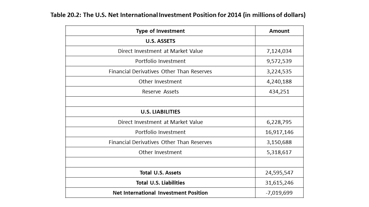
 Foreign exchange rates simply tell us what the price of one nation’s currency is in terms of another nation’s currency. For example, on Tuesday, January 15, 2008, the price of one Euro was about $1.4842. By Wednesday, January 16, 2008, the price of a Euro was only $1.4643. The price of a Euro had thus fallen from one day to the next. The prices of the Chinese Yuan and the U.K. Pound had also fallen. The Yuan fell from $0.1382 to $0.1381, and the U.K. Pound fell from $1.9671 to $1.9638. All these currencies fell in value relative to the U.S. dollar over the course of these two days. When a currency’s value declines relative to another currency, we say that it has depreciated against the other currency.
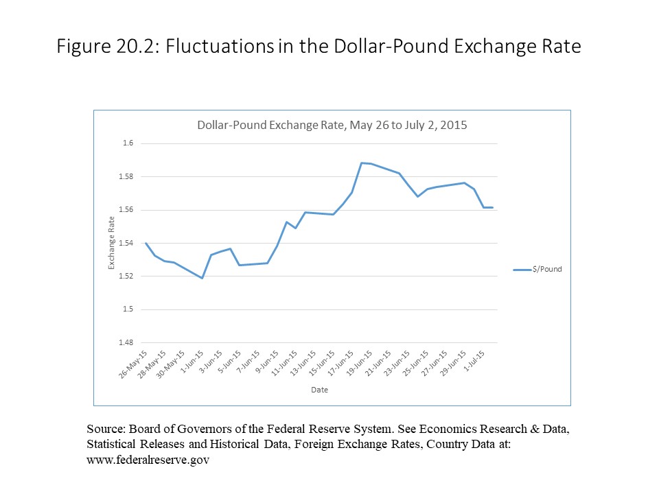
 The equilibrium exchange rate of $1.4842 per Euro occurs where the quantity demanded and the quantity supplied of Euros are equal. If the exchange rate exceeds this level, then a surplus of foreign exchange will exist, and competition will drive the exchange rate down. If the exchange rate falls short of this level, then a shortage of foreign exchange will exist, and competition will drive the exchange rate up. The equilibrium quantity exchanged of Euros (€*) is also determined as competition brings about the equilibrium outcome in the market.
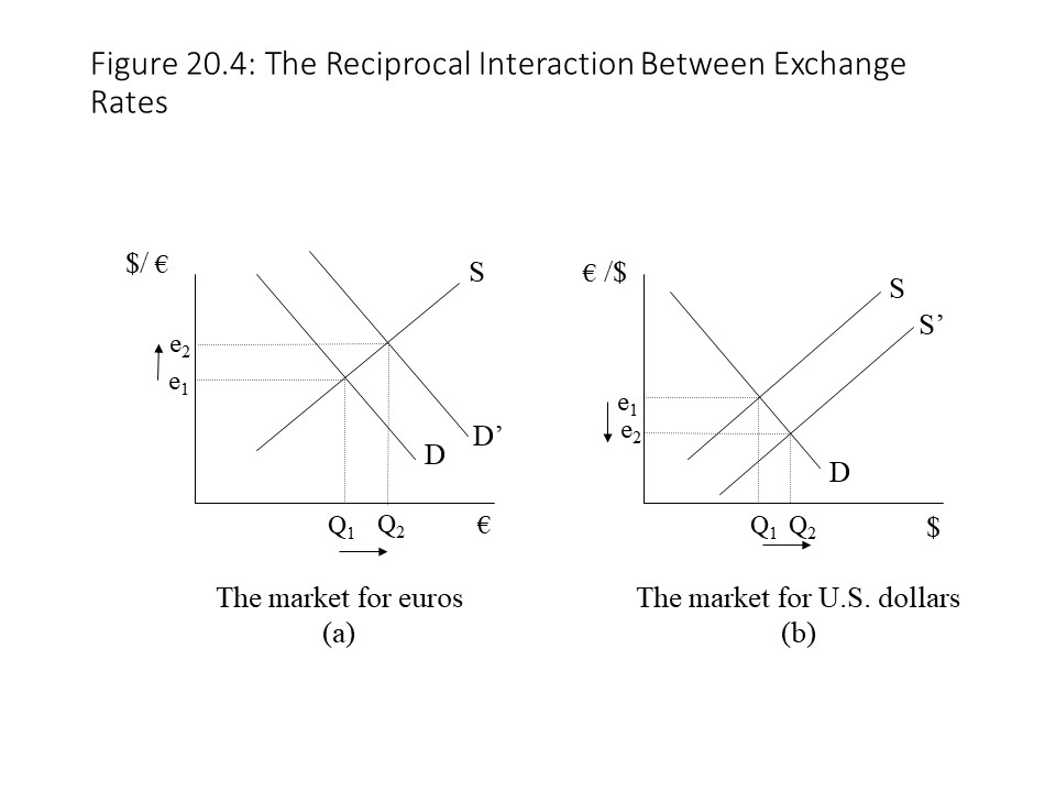 The rightward shift of demand in the market for Euros corresponds to a rightward shift of supply in the market for U.S. dollars. As mentioned previously, buyers of Euros are sellers of U.S. dollars when we are discussing the dollar-euro and euro-dollar markets. The consequence is an appreciation of the Euro and a depreciation of the U.S. dollar, reflecting the reciprocal connection between these exchange rates. The equilibrium quantities exchanged of both Euros and U.S. dollars increase as well.
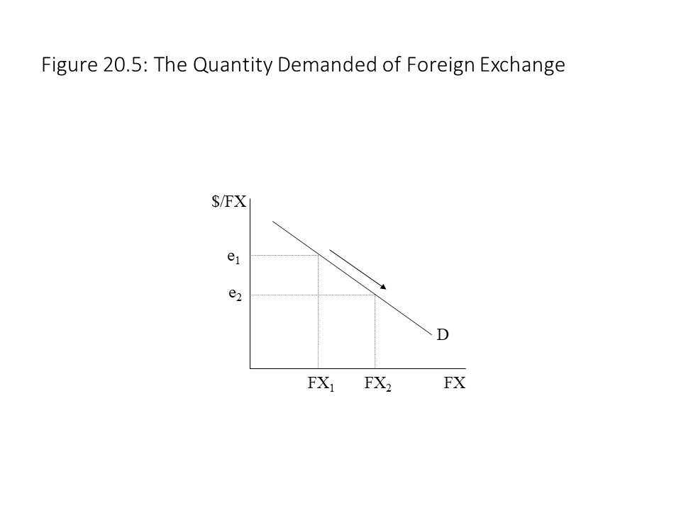 As the exchange rate falls, the foreign currency becomes cheaper and the quantity demanded of foreign exchange rises. It is worth asking why the demand curve slopes downward in this case.[4] When we learned about product markets, it seemed obvious that a lower price for a good, like apples, would lead to a rise in the quantity demanded of apples, ceteris paribus. As the price falls, other things the same, consumers are willing and able to buy more apples. The problem is that the explanation does not seem quite so obvious in the case of a foreign currency. After all, we do not eat Euros and so a lower price may not seem like it would automatically lead to increased purchases. Although we do not eat foreign currencies, they are useful as a means to an end. That is, if we wish to buy foreign goods and services, then we need to buy foreign currencies. Therefore, when the price of a foreign currency declines, we buy more of it because it allows us to purchase more foreign goods and services. That is, foreign goods and services become cheaper when the exchange rate ($/FX) falls and so we purchase more of the foreign currency.
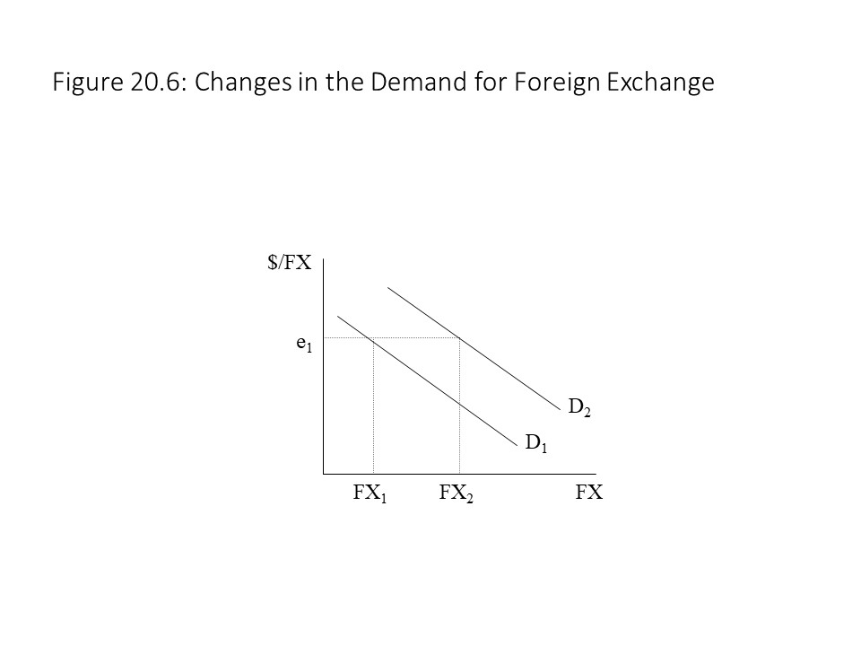 In Figure 20.6 a rise in the quantity demanded of foreign exchange occurs at every possible exchange rate. Which factors might cause such a shift of the demand curve for foreign exchange?[6] The first factor that we will consider is a change in consumers’ preferences in the home nation. For example, let’s suppose that American consumers develop a stronger preference for a specific nation’s automobiles. In that case, the demand for that foreign currency will increase. That is, the quantity demanded of the foreign currency will rise at every exchange rate, resulting in a rightward shift of the demand curve. If for some reason, the preferences of Americans changed such that they wanted fewer automobiles at each exchange rate, then the demand curve would shift to the left.
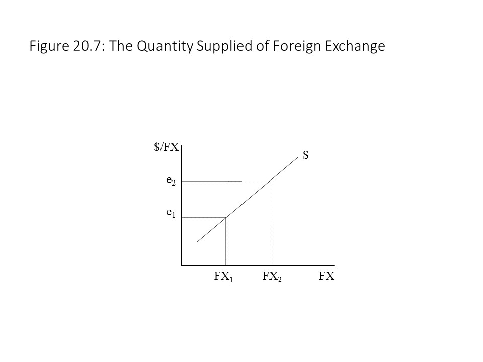 As the exchange rate rises, the foreign currency becomes more expensive and the quantity supplied of foreign exchange rises. It is worth asking why the supply curve slopes upward in this case. When we learned about product markets, it seemed obvious that a higher price for a good, like apples, would lead to a rise in the quantity supplied of apples, ceteris paribus. As the price rises, other things the same, producers are willing and able to sell more apples. In the case of foreign exchange markets, sellers are willing and able to sell more foreign exchange because when they sell foreign exchange, they acquire U.S. dollars, which are useful as a means to an end. That is, if foreigners wish to buy American goods and services, then they need to buy U.S. dollars. Therefore, when the price of a foreign currency rises, they sell more of it because it allows them to purchase more American goods and services. That is, American goods and services become cheaper when the exchange rate ($/FX) rises and so they sell more of the foreign currency.
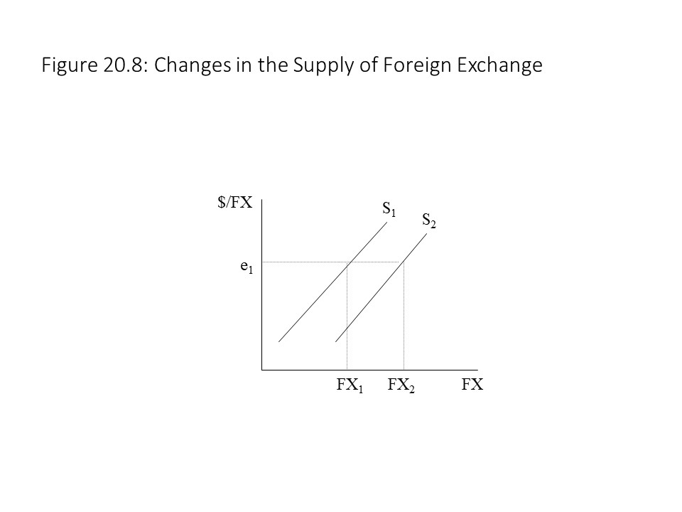 In Figure 20.8 a rise in the quantity supplied of foreign exchange occurs at every possible exchange rate. Which factors might cause such a shift of the supply curve for foreign exchange? Just as in the case of the demand for foreign exchange, it is possible that consumer preferences in the foreign nation change. For example, let’s suppose that foreign consumers develop a stronger preference for American automobiles. In that case, the supply of the foreign currency will increase. That is, the quantity supplied of the foreign currency will rise at every exchange rate, resulting in a rightward shift of the supply curve. If for some reason, the preferences of foreigners changed such that they wanted fewer American automobiles at each exchange rate, then the supply curve would shift to the left.
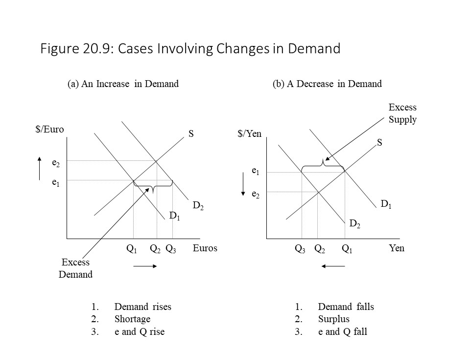
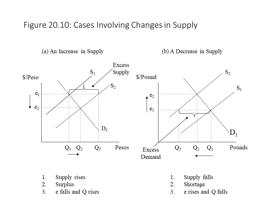
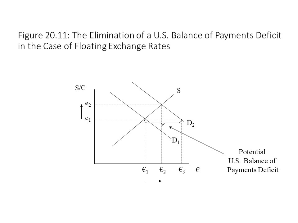 The increase in the demand for Euros creates a shortage of Euros, but we can also give another interpretation to the shortage. The quantity demanded of Euros (€3) at the initial exchange rate of e1 exists because Americans wish to buy European imports of goods and services, European assets, and Euros for speculation. These demands are potential debits in the U.S. Balance of Payments. At the same time, the quantity supplied of Euros (€1) at the initial exchange rate of e1 exists because Europeans wish to purchase American exports of goods and services, American assets, and U.S. dollars for speculation. These supplies are potential credits in the U.S. Balance of Payments. Therefore, the difference between the quantity demanded of Euros and the quantity supplied of Euros may be interpreted as the potential excess of debits over credits in the U.S. Balance of Payments. That is, it reflects a potential balance of payments deficit. Of course, the overall balance of payments must be balanced. Therefore, we need an explanation for how this discrepancy is resolved.
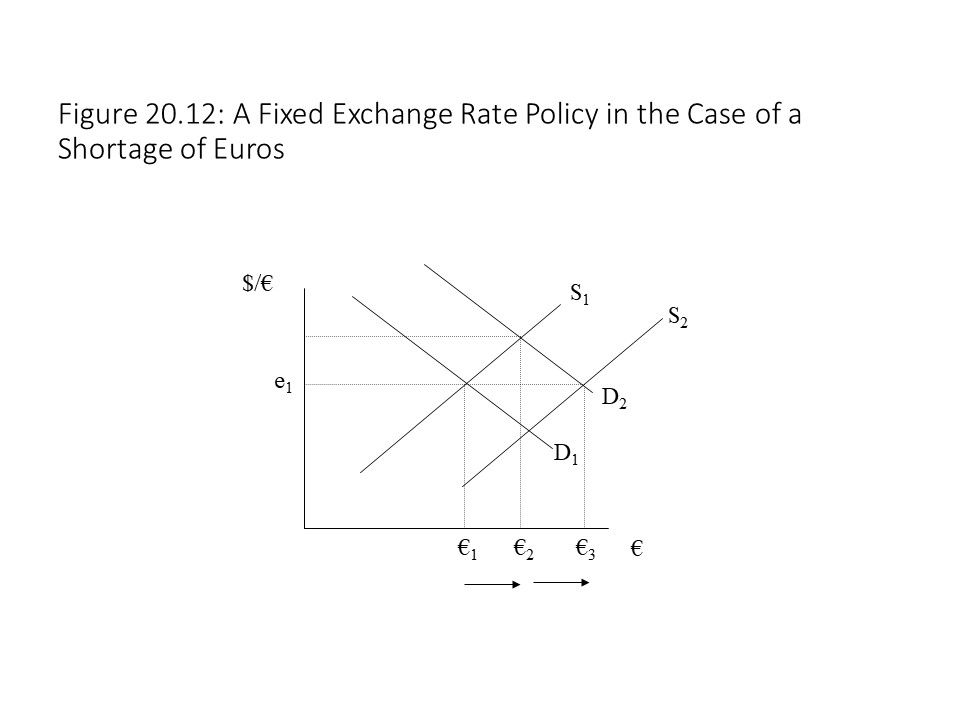 This increase in supply will allow the central bank to maintain an exchange rate of e1. It will also eliminate the potential for a balance of payments deficit because credits and debits will be equal. The difference has been made up with the expenditure of official reserves. That is, Euros held in reserve with the central bank have been spent in the foreign exchange market. These sales of Euros and purchases of U.S. dollars count as credits in the U.S. Balance of Payments. The result is an overall payments balance and a fixed exchange rate. In other words, since exports of U.S. goods, services, and assets are not sufficient to purchase imports of goods, services, and assets, then the difference must be made up by drawing down official reserves.
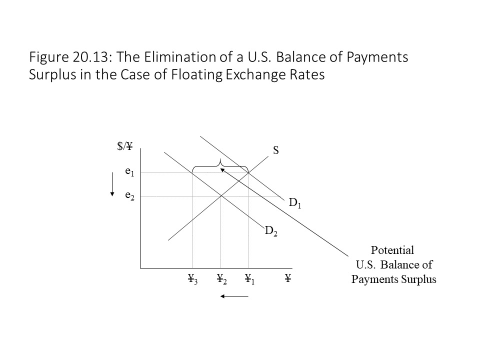 The decrease in the demand for Yen creates a surplus of Yen, but we can also give another interpretation to the surplus. The quantity supplied of Yen (¥1) at the initial exchange rate of e1 exists because Japanese consumers and investors wish to buy U.S. exports of goods and services, U.S. assets, and U.S. dollars for speculation. These supplies are potential credits in the U.S. Balance of Payments. At the same time, the quantity demanded of Yen (¥3) at the initial exchange rate of e1 exists because Americans wish to purchase Japanese imports of goods and services, Japanese assets, and Yen for speculation. These demands are potential debits in the U.S. Balance of Payments. Therefore, the difference between the quantity supplied of Yen and the quantity demanded of Yen may be interpreted as the potential excess of credits over debits in the U.S. Balance of Payments. That is, it reflects a potential balance of payments surplus. Of course, the overall balance of payments must be balanced. Therefore, just as before, we need an explanation for how this discrepancy is resolved.
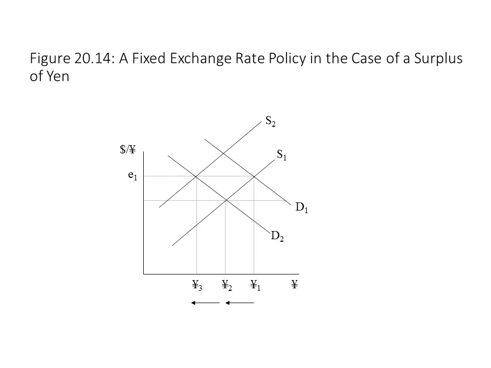 This decrease in supply will allow the central bank to maintain an exchange rate of e1. It will also eliminate the potential for a balance of payments surplus because credits and debits will be equal. The difference has been made up with an increase in U.S. official reserves. That is, Yen have been withdrawn from the foreign exchange market and added to official reserve assets. Because the supply of Yen represents potential credits in the U.S. Balance of Payments, when they are withdrawn, potential credits fall until they match debits. The result is an overall payments balance and a fixed exchange rate. In other words, since exports of U.S. goods, services, and assets exceed U.S. imports of Japanese goods, services, and assets, the surplus of Yen must be added to foreign exchange reserves if the exchange rate is to be kept at the same level.
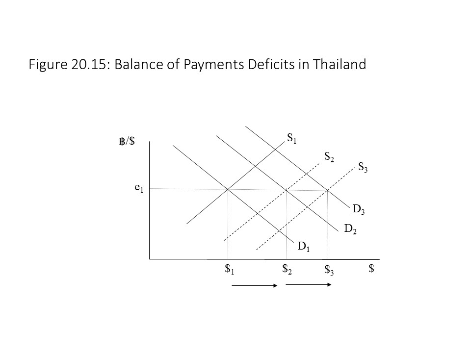
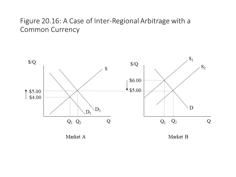 If we ignore transportation costs, it will not take long before some motivated individuals decide to purchase the commodity in market A and then sell the commodity in market B. The higher demand in market A will push up the equilibrium price in market A to $5 per unit, just as the higher supply in market B will push down the equilibrium price in market B to $5 per unit. Eventually, the prices will equalize, as shown in Figure 20.16. This practice of buying a commodity at a low price in one location and selling it at a higher price in another location is called arbitrage.
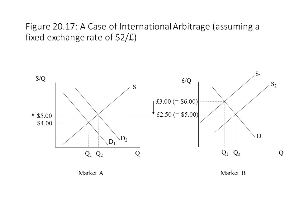 Because of the different currencies, it is necessary to convert one currency into the other so that we can compare prices. This conversion can only be carried out using the current exchange rate. Let’s assume that the pound-dollar exchange rate is £0.50/$ and that the dollar-pound exchange rate is $2/£. The reader should recall that each is simply the reciprocal of the other. Therefore, if the commodity is priced at £3 in the U.K., then its dollar price must be $6 (= £3 times $2/£).
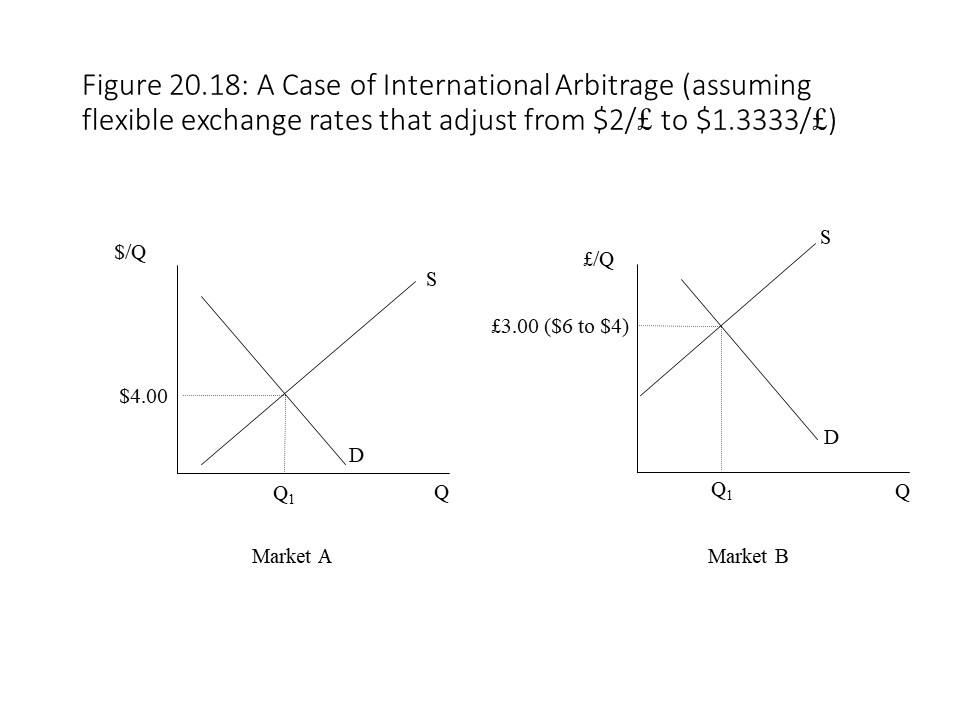 For commodities that are easily tradeable across nations, we should expect an outcome like what we have just described. For commodities that are not easily traded (e.g., services like haircuts), we should expect to observe more variation in purchasing power. That is, we should expect the prices to be quite different after we make the conversion into a common currency. Therefore, while this theory provides a useful starting point for thinking about international price adjustments, limits to its application exist, particularly where excessive transport costs interfere with arbitrage.
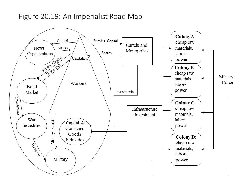
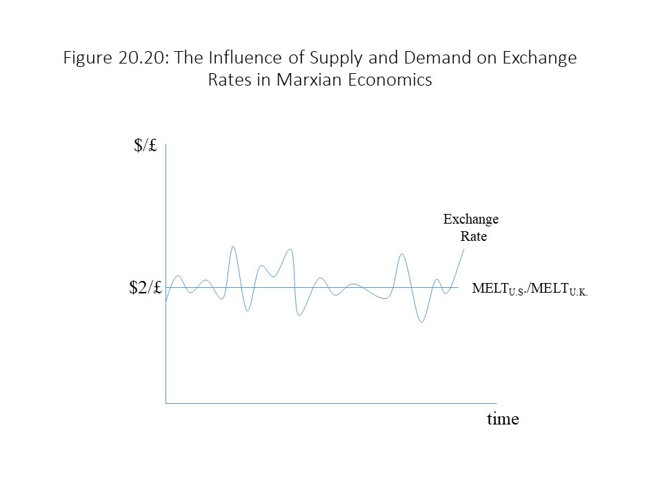 It should be noted that Marxian economists are interested in understanding the social relationships that give rise to the appearances they observe in the marketplace. This theory of exchange rate determination should be viewed only as a complement to the theory of imperialist finance that was developed in the previous section. The class conflict inherent in the vast network connecting the imperialist power with its colonies (or neo-colonies) is what ultimately concerns the Marxist. It is the focus because a solid understanding of it will assist in the revolutionary overthrow of the capitalist economic system that makes such relations possible.