The study of markets is a powerful, informative, and useful method for understanding the world around us, and interpreting economic events. The use of supply and demand allows us to understand how the world works, how changes in economic conditions affect prices and production, and how government policies and programs affect prices, producers, and consumers. A huge number of diverse and interesting issues can be usefully analyzed using supply and demand.
Supply
The Supply of a good represents the behavior of firms, or producers. Supply refers to how much of a good will be produced at a given price.
Supply = The relationship between the price of a good and quantity supplied, ceteris paribus.
Notice the important term, “ceteris paribus” at the end of the definition of supply. Recall the complexity of the real world, and how economists must simplify the world to understand it. Use of the concept, ceteris paribus, allows us to understand the supply of a good. In the real world, there are numerous forces affecting the supply of a good: weather, prices, input prices, just to name a few.
Ceteris Paribus = Holding all else constant (Latin).
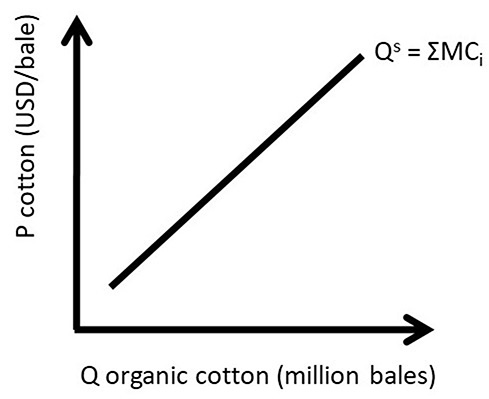
When studying supply, we seek to isolate the relationship between the price and quantity supplied of a good. We must hold everything else constant (ceteris paribus) to make sure that the other supply determinants are not causing changes in supply. An example is the supply of organic cotton. Patagonia spearheaded the movement into using organic cotton in the production of clothing. Nike and other clothing manufacturers are increasing organic clothing production to meet the growing demand for this good. Interestingly, conventional (non-organic) cotton is the most chemical-intensive field crop, and can result in agricultural chemical runoff in the soil and groundwater. A small but convicted group of consumers are willing to pay high premiums for clothing made with organic cotton, to reduce the potential environmental damage from agricultural chemicals used in cotton production. Notice that this graph has two items on each axis: (1) a label, and (2) units. Every graph drawn must have both labels and units on each axis to effectively communicate what the graph is about.
Figure \(\PageIndex{1}\) Market Supply Curve of Organic Cotton
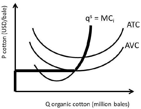
The supply curve seen in Figure \(\PageIndex{1}\) is a market supply curve, as it represents the entire market of organic cotton (note that cotton is sold in bales). The market supply curve was derived by horizontal summation all of the individual firm supply curves. This is indicated by the notation \(Q^s = ΣMC_i\) in Figure \(\PageIndex{1}\). The individual firm supply curve is the firm’s marginal cost curve \((MC)\) for all prices above the shut down point, and equal to zero for all prices below the shut down point. The shut down point is the minimum point on the firm’s average variable cost curve \((AVC)\), as shown in Figure \(\PageIndex{2}\)
Since the market supply curve is the sum of all of the individual firms’ marginal cost curves \((ΣMC_i)\), the market supply curve represents the cost of production: the total amount that a business firm must pay to produce a given quantity of a good.
There are three properties of a market supply curve.
Figure \(\PageIndex{2}\) Individual Firm Supply Curve of Organic Cotton
Properties of Supply
Upward-sloping: if price increases, quantity supplied increases,
\(Q^s= f(P)\), and
Ceteris Paribus, Latin for “holding all else constant.”
The first property reflects the Law of Supply, which states that there is a direct relationship between price and quantity supplied.
Law of Supply = There is a direct, positive relationship between the price of a good and the quantity supplied, ceteris paribus.
The second property demonstrates that price \((P)\) is the independent variable, and quantity supplied \((Q^s)\) is the dependent variable. Graphs of supply and demand are drawn “backward” with the independent variable \((P)\) on the vertical axis. In all other fields of mathematics and science, when a function such as \(y=f(x)\) is graphed, the independent variable \((x)\) appears on the horizontal axis, and the dependent variable \((y)\) is drawn on the vertical axis. Supply and demand graphs are drawn, “backwards” due to economist Alfred Marshall, who drew the original supply and demand graphs this way in his Principles of Economics book in 1890. The third property reflects the need to simplify all of the determinants of supply to isolate the relationship between price and quantity supplied, using the ceteris paribus assumption.
The Determinants of Supply
There are numerous determinants of supply, so we will focus on five important ones. The most important supply determinant, or driver, is price \((P)\). Other determinants include input prices \((Pi)\), the prices of related goods \((Pr)\), technology \((T)\), and government taxes and subsidies \((G)\).
\[ Q^s = f(P, Pi, Pr, T, G) \label{1.1}\]
To draw a supply curve, we focus on the most important determinant of supply: the good’s own price. We hold all of the other determinants constant. To show this in equation form, we use a vertical bar to designate ceteris paribus: all variables that appear to the right of the vertical bar are held constant. Equation \ref{1.2} shows the relationship between quantity supplied and price, holding all else constant. This relationship is the market supply curve in Figure \(\PageIndex{1}\) and in supply and demand graphs.
\[Q^s = f(P| Pi, Pr, T, G) \label{1.2}\]
Input prices \((Pi)\) are important determinants of supply, since the supply curve represents the cost of production. Prices of related goods \((Pr)\) represent prices of substitutes and complements in production. Substitutes in production are goods that are produced either/or, such as corn and soybeans. One land parcel can be used to grow either corn or soybeans. Complements in production are goods that are produced together in a fixed ratio. Beef and leather are complements in production. Technology \((T)\) is major driver of supply, as new methods and techniques become available, they increase the amount of food produced. Technological change allows more output to be produced with the same level of inputs. Restated, the same level of output can be produced with fewer inputs. Government policies and programs \((G)\) can shift the supply of a good through taxes or subsidies.
Movements Along vs. Shifts In Supply
The supply curve represents the mathematical relationship between the price and quantity supplied of a good. Therefore, when a good’s own price changes, it is as a movement along the supply curve. When any of the other supply curve determinants change, it will shift the entire curve.
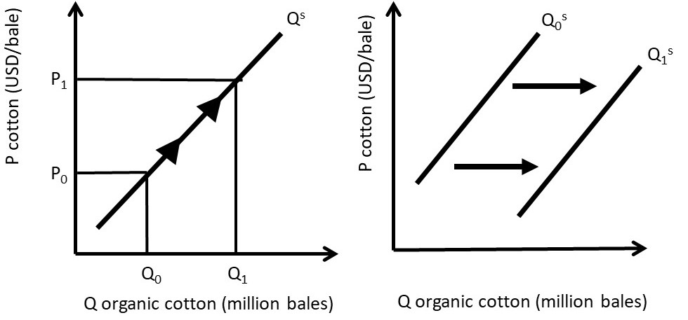
A movement along a supply curve, caused by a change in the good’s own price, is called a change in quantity supplied (left panel, Figure \(\PageIndex{3}\)). A shift in the supply curve, caused by a change in any supply determinant other than the good’s own price, is called a change in supply (right panel, Figure \(\PageIndex{3}\)). The change in supply shown in Figure \(\PageIndex{3}\) is an increase in supply, since it increases the quantity supplied at any given price.
Figure \(\PageIndex{3}\) Movement Along and Shift in the Supply of Organic Cotton
Notice that the supply curve has shifted down, yet this represents an increase in supply. The supply change is measured on the horizontal axis, so a movement from left to right represents an increase in supply. The shift shown could be the impact of technological change on organic cotton supply: suppose that biotechnology allows for higher yielding varieties of organic cotton.
Demand
The Demand of a good represents the behavior of households, or consumers. Demand refers to how much of a good will be purchased at a given price.
Demand = The relationship between the price of a good and quantity demanded, ceteris paribus.
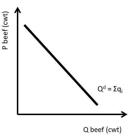
Figure 1.4 shows the market demand curve for beef \((Q^d)\), derived by the summation of all individual consumers demand curves \((Σq_i)\). Note that beef is measured in units of one hundred pounds, or a “hundredweight” (cwt).
Demand represents the willingness and ability of consumers to purchase a good. As with supply, there are three properties of demand.
Figure \(\PageIndex{4}\) Market Demand for Beef
Properties of Demand
Downward-sloping: if price increases, quantity demanded decreases,
\(Q^d= f(P)\), and
Ceteris Paribus, Latin for holding all else constant.
The first property reflects the Law of Demand, which states that if the price of a good increases, the quantity demanded of that good decreases, holding all else constant.
Law of Demand = There is an inverse relationship between the price of a good and the quantity supplied, ceteris paribus.
The Law of Demand is one of the major “take home messages” of economic principles. Price increases lead to smaller quantities of goods purchased. The Law of Demand does not say that all consumers will stop buying a good, it says that at least some consumers will decrease consumption of the good. The magnitude of the decrease will depend on the price elasticity of demand for the good, as will be discussed in Section 1.4 below.
The Determinants of Demand
There are numerous demand shifters, or determinants of demand. Six of the most important determinants are included in the demand equation in Equation \ref{1.3}. The good’s own price \((P)\) is the most important determinant. Demand is also influenced by: the price of related goods \((Pr)\), futures prices \((Pf)\), income \((I)\), tastes and preferences \((T)\), and government programs and policies \((G)\).
\[ Q^d = f(P, Pr, Pf, I, T, G) \label{1.3}\]
Related goods include substitutes and complements in consumption. Substitutes in consumption are goods that are purchased either/or, such as hot dogs and hamburgers. If the price of hot dogs increases, at least some consumers will shift out of hot dogs and into hamburgers. Complements in consumption are goods that are consumed together, for example hot dogs and hot dog buns. If the price of hot dogs increases, consumers will purchased fewer hot dogs and fewer buns.
Expectations of future prices \((Pf)\) have a large influence on consumption decisions today. If the price of corn was expected to increase in the future, corn demand would increase today, as corn buyers would seek to buy prior to the price increase. This would allow traders to “buy low and sell high,” providing profit from arbitrage across time.
Income \((I)\) can have a large impact on purchase decisions. Cars, houses, and other expensive items will be affected by changes in income. Inexpensive items such as used clothes or ramen noodles are also influenced greatly by income changes. During the great recession of 2008-2010, Walmart had high profit levels, while boat manufacturers and country clubs lost profits due to significant decreases in income.
Tastes and preferences \((T)\) shift the demand for goods and services based on the diverse wants, needs, and desires of consumers in the market. Taxes and subsidies, as well as other government programs, policies, and regulations \((G)\) influence demand, sometimes significantly. Government programs and policies will be explored in Sections 1.4 through 1.6, and in Chapter 2 below.
To draw a demand curve, the most important determinant of demand is isolated: the good’s own price. We hold all of the other determinants constant, ceteris paribus.
\[ Q^d = f(P | Pr, Pf, I, T, G) \label{1.4}\]
Movements Along vs. Shifts In Demand
The demand curve represents the mathematical relationship between the price and quantity demanded of a good. Therefore, when a good’s own price changes, it is depicted as a movement along the demand curve. When any of the other demand curve determinants change, it will shift the entire curve.
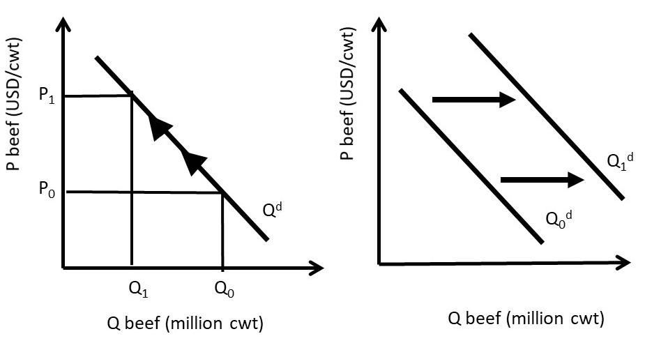
Figure \(\PageIndex{5}\) Movement Along and Shift in the Demand for Beef
As with supply, if the good’s own price changes, it results in a movement along the demand curve, called a change in quantity demanded. If any other demand determinant changes, it causes a shift in demand, called a change in demand. The shift shown in the right panel of Figure \(\PageIndex{5}\) is an increase in demand, since the demand curve has shifted upward and to the right.
Supply and demand form the foundation for the study of markets. Markets are defined as the interaction of supply and demand. Market analysis is the core concept and foundation of all of economics, and will be explored in the next section.