
1.3: Markets - Supply and Demand
- Last updated
- Save as PDF
- Page ID
- 43147

In the previous section, supply and demand were introduced and explored separately. In what follows, the interaction of supply and demand will be presented. The market mechanism is a useful and powerful analytical tool. The market model can be used to explain and forecast movements in prices and quantities of goods and services. The market impacts of current events, government programs and policies, and technological changes can all be evaluated and understood using supply and demand analysis. Markets are the foundation of all economics!
A market equilibrium can be found at the intersection of supply and demand curves, as illustrated for the wheat market in Figure \(\PageIndex{1}\). An equilibrium is defined as, “a point from which there is no tendency to change.” Wheat is traded in units of metric tons (MT), or 1000 kilograms, equal to approximately 2,204.6 pounds.
Equilibrium = a point from which there is no tendency to change.
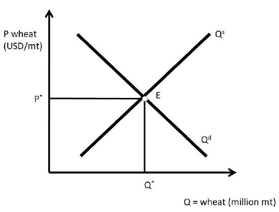
Point \(E\) is the only equilibrium in the wheat market shown in Figure \(\PageIndex{1}\). At any other price, market forces would come into play, and bring the price back to the equilibrium market price, \(P^*\). At any price higher than \(P^*\), such as \(P’\) in Figure \(\PageIndex{2}\), producers would increase the quantity supplied to \(Q_1\) million metric tons of wheat, and consumers would decrease the quantity demanded to \(Q_0\) million metric tons of wheat. A surplus would result, since quantity supplied is greater than quantity demanded \((Q_1 > Q_0)\).
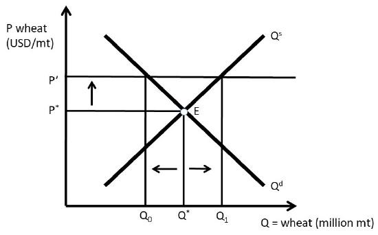
A wheat surplus such as the one shown in Figure \(\PageIndex{2}\) would bring market forces into play since \(Q^s \neq Q^d\). Wheat producers would lower the price of wheat in order to sell it. It would be preferable to earn a lower price than to let the surplus go unsold. Consumers would increase the quantity demanded along \(Q^d\) and producers decrease the quantity supplied along \(Q^s\) until the equilibrium point \(E\) was reached. In this way, any price higher than the market equilibrium price will be temporary, as the resulting surplus will bring the price back down to the equilibrium price \(P^*\).
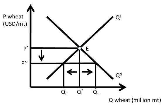
Market forces also come into play at prices lower than the equilibrium market price, as shown in Figure \(\PageIndex{3}\). At the lower price \(P’’\), producers reduce the quantity supplied along \(Q^s\) to \(Q_0\), and consumers increase the quantity demanded to \(Q_1\). A shortage occurs, since the quantity demanded is greater than the quantity supplied \(Q_1 > Q_2\). The shortage will bring market forces into play, as consumers will bid up the price in order to purchase more wheat and producers will produce more wheat along \(Q^s\). This process will continue until the market price returns to the equilibrium market price, \(P^*\).
The market mechanism that results in an equilibrium price and quantity performs a truly amazing function in the economy. Markets are self-regulating, since no government intervention or coercion is needed to achieve desirable outcomes. If there is a drought, the price of wheat will rise, causing more resources to be devoted to wheat production, which is desirable, since wheat is in short supply during a drought. If good weather causes a surplus, the price will fall, causing wheat producers to shift resources out of wheat and into more profitable opportunities. In this fashion, the market mechanism allows voluntary trades between willing parties to allocate resources to the highest return. Efficiency of resource use and high incomes are a feature of market-based economies.
Although markets provide huge benefits to society, not everyone wins from free market economies, and market changes over time. Price increases help producers, but hurt consumers. Technological change has provided lowered food prices enormously over time, but has led to farm and ranch consolidation, and the large migration of farmers and their families out of rural regions and into urban areas.
The market graphs of supply and demand are based on the assumption of perfectly competitive markets. Perfect competition is an ideal state, different from actual market conditions in the real world. Once again, economists simplify the complex real world in order to understand it. We will begin with the extreme pure case of perfect competition, and later introduce realism into our analysis.
Competitive Market Properties
A competitive market has four properties:
- homogeneous product,
- numerous buyers and sellers,
- freedom of entry and exit, and
- perfect information.
The first property of perfect competition is a homogeneous product. This means that the consumer can not distinguish any differences in the good, no matter which firm produced it. Wheat is an example, as it is not possible to determine which farmer produced the wheat. A John Deere tractor is an example of a nonhomogeneous good, since the brand is displayed on the machine, not to mention the company’s well known green paint and deer logo.
The assumption of numerous buyers and sellers means something specific. The word, “numerous” refers to an industry so large that each individual firm can not affect the price. Each firm is so small relative to the industry that it is a price taker.
Freedom of entry and exit means that there are no legal, financial, or regulatory barriers to entering the market. A wheat market allows anyone to produce and sell wheat. Attorneys and physicians, however, do not have freedom of entry. To practice law or medicine, a license is required.
Perfect information is an assumption about industries where all firms have access to information about all input and output prices, and all technologies. There are no trade secrets or patented technologies in a perfectly competitive industry. These four properties of perfect competition are stringent, and do not reflect real-world industries and markets. Our study of market structures in this course will examine each of these properties, and use them to define industries where these properties do not hold. Competitive markets have a number of attractive properties.
Outcomes of Competitive Markets
Competitive markets result in desirable outcomes for economies. A competitive market maximizes social welfare, or the total amount of well-being in a market. Competitive markets use voluntary exchange, or mutually beneficial trades, to achieve this result. In a market-based economy, no one is forced, or coerced, to do anything that they do not want to do. In this way, all trades are mutually beneficial: a producer or consumer would never make a trade unless it made him or her better off. This idea will be a theme throughout this course: free markets and free trade lead to superior economic outcomes.
It should be emphasized that free markets and free trade are not perfect, since there are negative features associated with markets and capitalism. Income inequality is an example. Markets do not solve all of society’s problems, but they do create conditions for higher levels of income and wealth than other economic organizations, such as a command economy (as found in a communist or fascist nation). There are winners and losers to market changes. An example is free trade. Free trade lowers prices for consumers, but often causes hardships for producers in importing nations. Similarly, open borders allow immigrants to improve their conditions and earnings by moving from low-income nations to high-income nations such as the United States (US) or the European Union (EU). Workers in the US and the EU will face competition from a larger labor supply, causing reductions in wages and salaries. A simple example of markets is an increase in the price of corn. Corn producers are made better off, but livestock producers, the major buyers of corn, are made worse off. Thus, the market shifts that allow prosperity also create winners and losers in a free market economy.
Supply and Demand Shift Examples
Given our knowledge of markets and the market mechanism, current events and policies can be better understood.
Demand Increase
China was a command economy until 1986. At that time, the government introduced the Household Responsibility System, which allowed farmers to earn income based on how much agricultural output they produced. The new policy worked very well, and China moved from being a net food importer to a net food exporter. Soon, the policy was extended to all industries, and China was on its way to a market-based economy. The result has been a truly unprecedented increase in income. China has gone from a low income nation to a middle income nation, and the rates of economic growth are higher than any nation in history. And, these growth rates are for the world’s most populous nation: 1.4 billion people (for comparison, the United States (USA) has approximately 326 million people).
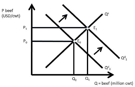
This historical income growth in China has been good for US farmers and ranchers. As incomes increase, consumers shift out of grain-based diets such as rice and wheat, and into meat. There has been a large increase in beef consumption in China as incomes increased. This is an increase in the demand for US beef, as shown in Figure \(\PageIndex{4}\). The units for beef are hundredweight (cwt), or one hundred pounds. This is called an increase in demand (do you remember why this is not an increase in quantity demanded?). The outward shift in demand results in a movement from equilibrium \(E_0\) to \(E_1\). The movement along the supply curve for beef is called an increase in quantity supplied. The equilibrium market price increases from \(P_0\) to \(P_1\), and the equilibrium market quantity increases from \(Q_0\) to \(Q_1\). An increase in demand results in higher prices and higher quantities. As a result, the best way to increase profitability for a firm is to increase demand.
Interestingly, income growth in China is beneficial to not only US beef producers, who face an increased demand for beef, but also for grain farmers in the USA. The major input into the production of beef is corn, sorghum (also called milo), and soybeans. These grains are fed to cattle in feedlots. Seven pounds of grain are required to produce one pound of beef. Therefore, any increase in the global demand for beef will result in an increase in demand for beef, and a large increase in the demand for feed grains.
Demand Decrease
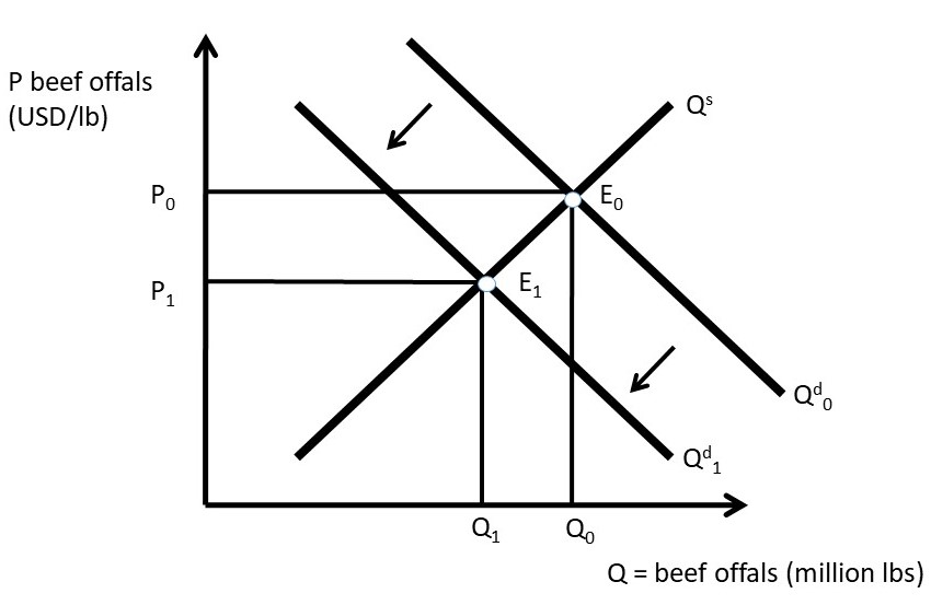
In the United States, the demand for beef offals (tripe, tongue, heart, liver, etc.) has decreased in the past few decades. As incomes increase, consumers shift out of these goods and into more expensive meat products such as hamburger and steaks. The demand for offals has decreased as a result, as in Figure \(\PageIndex{5}\). This is a decrease in demand (shift inward), and a decrease in quantity supplied (movement along the supply curve). The outcome is a decrease in the equilibrium market price and quantity of beef offals.
Supply Decrease
A large share of citrus fruit in the US is grown in Florida and California. If there is bad weather in either State, the market for oranges, lemons, limes, and grapefruit is affected. An early freeze can damage the citrus fruit, resulting in a decrease in supply (Figure \(\PageIndex{6}\)).
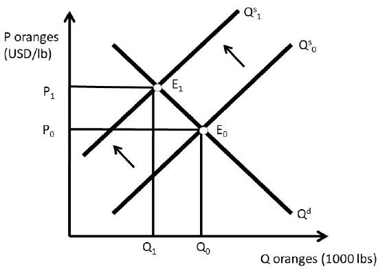
The supply decrease is a shift in the supply curve to the left, resulting in a movement along the demand curve: a decrease in quantity demanded. The equilibrium price increases, and the equilibrium quantity decreases.
Supply Increase
Technological change is a constant in global agriculture. Science and technology has provided more output from the same levels of inputs for many decades, and especially since 1950. Biotechnology in field crops has been a recent enhancement in the world food supply. Biotechnology is also referred to as genetically modified organisms (GMOs). Although GMOs are often in the news media as a potential health risk or environmental risk, they have been produced and consumed in the US for many years, with no documented health issues. However, the herbicide glyphosate has been determined to be a carcinogen in recent studies. Glyphosate is the ingredient in “RoundUp,” a widely used herbicide in corn and soybean production. Genetically modified corn and soybeans are resistant to this herbicide, so it has been used extensively since the introduction of GM crops. Biotechnology has increased the availability of food enormously, and is considered the largest technological change in the history of agriculture. The impact of biotechnology is shown in Figure \(\PageIndex{7}\).
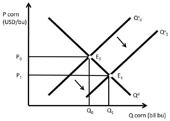
Biotechnology results in an increase in supply, the rightward shift in the supply curve. This supply shift results in a movement along the demand curve, an increase in quantity demanded. The equilibrium quantity increases, and the equilibrium price decreases. It may seem that the decrease in price is bad for corn producers. However, in a global economy, this keeps the US competitive in global grain markets. Since a large fraction of US grain crops are exported, this provides additional income to the corn industry.
Mathematics of Supply and Demand
The above market analyses are qualitative, or non-numerical. Numbers can be added to the supply and demand graphs to provide quantitative results. The numbers used here are simple, but can be replaced with actual estimates of supply and demand to yield important and interesting quantitative results to market events.
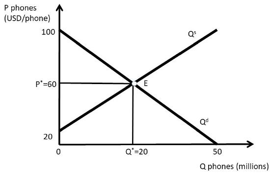
As an example, consider the phone market. Let the inverse demand for phones be given by Equation \ref{1.5}. The equation is called, “inverse” because the independent variable \((P)\) appears on the left-hand side and the dependent variable \((Q^d)\) appears on the right hand side. Traditionally, the independent variable \((x)\) is on the right, and the dependent variable \((y)\) is on the left. We use inverse supply and demand equations for easier graphing, since \(P\) is on the vertical axis, typically used for the dependent variable (can you remember why these graphs are backwards?).
\[P = 100 – 2Q^d \label{1.5}\]
In the inverse demand equation, \(P\) is the price of phones in USD/unit, and \(Q\) is the quantity of phones in millions. The inverse supply equation is given in Equation \ref{1.6}.
\[P = 20 + 2Q^s\label{1.6}\]
These examples of inverse supply and demand functions are called “price-dependent” for ease of graphing. The equations can be quickly and easily inverted to “quantity-dependent” form. To do this, use simple algebra to isolate \(Q^d\) or \(Q^s\) on the left-hand side of the equations.
To find equilibrium, set \(Q^s = Q^d = Q^e\). This is the point where the market “clears,” and supply is equal to demand. By inspection of the market graph (Figure \(\PageIndex{8}\)), there is only one price where this can occur: the equilibrium price: \(P^e\).
\[\begin{align*} P &= 100 – 2Q^e = 20 + 2Q^e\\ 80 &= 4Q^e\\ Q^e &= 20 \end{align*}\]
To find the equilibrium price, plug \(Q^e\) into the inverse demand equation:
\[P^e = 100 – 2Q^e = 100 – 2*20 = 100 – 40 = 60.\]
This result can be checked by plugging \(Q^e = 20\) into the inverse supply equation:
\[P^e = 20 + 2Q^e = 20 + 2*20 = 20 + 40 = 60\]
The equilibrium price and quantity of phones are:
\[P^e = \text{ USD } 60\text{/phones, and } Q^e = 20 \text{ million phones.}\]
Notice that these equilibrium values have both labels (phones) and units.
We will be using quantitative market analysis throughout the rest of the course. If you have any questions about how to graph the functions, or how to solve for equilibrium price and quantity, be sure to review the material in this chapter carefully. We will be using these graphs throughout our study of market structures!