2.1: Price Ceiling

In some circumstances, the government believes that the free market equilibrium price is too high. If there is political pressure to act, a government can impose a maximum price, or price ceiling, on a market.

Price Ceiling = A maximum price policy to help consumers.

A price ceiling is imposed to provide relief to consumers from high prices. In food and agriculture, these policies are most often used in low-income nations, where political power is concentrated in urban consumers. If food prices increase, there can be demonstrations and riots to put pressure on the government to impose price ceilings. In the United States, price ceilings were imposed on meat products in the 1970s under President Richard M. Nixon. Price ceilings were also used for natural gas during this period of high inflation. It was believed that the cost of living had increased beyond the ability of family earnings to pay for necessities, and the market interventions were used to make beef, other meat, and natural gas more affordable.

Price ceilings are often imposed on housing prices in US urban areas. Rent control has been a longtime feature in New York City, where rent-controlled apartments continue to have low rental rates relative to the free market rate. The boom in the software industry has increased housing prices and rental rates enormously in the San Francisco Bay Area, Seattle, and the Puget Sound region. Rent control is being considered in both places to make San Francisco and Seattle more affordable for middle-class workers.

Welfare Analysis

Welfare analysis can be used to evaluate the impacts of a price ceiling. In what follows, we will compare a baseline free market scenario to a policy scenario, and compare the benefits and costs of the policy relative to the baseline of free markets and competition. Consider the price ceilings imposed on the natural gas markets. The purpose, or objective, of this policy was to help consumers. We will see that the policy does help some consumers, but makes other consumers worse off. The policy also hurts producers.

This unanticipated outcome is worth restating: price ceilings help some consumers, but hurt other consumers. All producers are made worse off. This outcome is not the intent of policy makers. Economists play an important role in the analysis and communication of policy outcomes to policy makers.

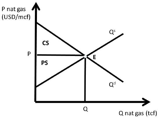
The baseline scenario for all policy analysis is free markets. Figure \(\PageIndex{1}\) shows the free market equilibrium for the natural gas market. The quantity of natural gas is in trillion cubic feet (tcf) and the price of natural gas in in dollars per million cubic feet (USD/mcf).

Social welfare is maximized by free markets, because the size of the welfare area \(CS + PS\) is largest under the free market scenario. As we will see, any government intervention into a market will necessarily reduce the total level of surplus available to consumers and producers. All price and quantity policies will help some individuals and groups, hurt others, and have a net loss to society. Policy makers typically ignore or downplay individuals and groups who are negatively affected by a proposed policy. The two triangles CS and PS are as large as possible in Figure \(\PageIndex{1}\).

Figure \(\PageIndex{1}\): Natural Gas Market Baseline Scenario: Free Markets

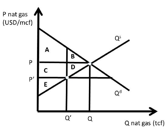
The price ceiling policy is evaluated in Figure \(\PageIndex{2}\), where \(P’\) is the price ceiling. Here, the government has passed a law that does not allow natural gas to be bought or sold at any price higher than \(P’ (P’ < P)\). For a price ceiling to have an impact, it must be “binding.” This occurs only when the price ceiling is set below the market price \((P’ < P)\). If the price ceiling were set above \(P (P’ > P)\), it would have no effect, since the good is bought and sold at the market price, which is below the price ceiling, and legally permissible. Such a law would not be binding on market transactions.

If the price ceiling is set at \(P’\), then the new equilibrium quantity under the price ceiling \((Q’)\) is found at the minimum of quantity demanded (\(Q^d\)) and quantity supplied (\(Q^s\)), as in Equation \ref{2.0}.

\[ Q^{\prime} = min(Q^s, Q^d) \label{2.0}\]

This condition states that the quantity at any nonequilibrium price \((P)\) will be the smallest of production or consumption. At the low price P’, producers decrease quantity supplied, and consumers increase quantity demanded, resulting in \(Q’ = Q^s\) (Figure \(\PageIndex{2}\)). This is the maximum amount of natural gas placed on the market, although consumers desire a much larger amount.

The first step in the welfare analysis is to assign letters to each area in the price ceiling graph. Next, the letters corresponding to the baseline free market scenario are recorded (initial, or baseline, values have a subscript 0), followed by the surpluses under the price ceiling (ending values have a subscript 1). Finally, the change from free markets to the price policy are calculated to conclude the qualitative analysis of a price ceiling. If the supply and demand curves have numbers (actual data) associated with them, a numerical analysis can be conducted.

The initial, baseline, free market values in the natural gas market at market equilibrium price \(P\) are:

\[CS_0 = A + B\nonumber\]

and

\[PS_0 = C + D + E.\nonumber\]

Social welfare is defined as the total amount of surplus available in the market, \(CS + PS\):

\[SW_0 = A + B + C + D + E.\nonumber\]

After the price ceiling is put in place, the price is P’, and the quantity is Q’. New surplus values are found in the same way as under free markets. Consumer surplus is the willingness to pay minus price actually paid, or the area beneath the demand curve and above the price line at the new price P’: (\(A + C\)). Producer surplus is the price received minus the cost of production, or the area above the supply curve and below the price line (\(E\)):

\[CS_1 = A + C,\nonumber\]

\[PS_1= E,\nonumber\]

and

\[SW_1 = A + C + E.\nonumber\]

Recall that social welfare (SW) is equal to the sum of all surpluses available in the market: \(SW = CS + PS\). The welfare analysis outcomes are found by calculating the changes in surplus:

\[\begin{align*} ΔCS &= CS_1 – CS_0 = + C – B \\[4pt] ΔPS &= PS_1 – PS_0 = – C – D \\[4pt] ΔSW &= SW_1 – SW_0 = – B – D \end{align*}\]

The results are fascinating, since the sign of the change in consumer surplus is ambiguous: the sign of \(\Delta CS\) depends on the relative magnitude of areas \(C and B\). If demand is elastic, and supply is inelastic, the price ceiling is more likely to yield a positive change in consumer surplus \((C > B)\). The policy makes some consumers better off, and some consumers worse off. The consumers located on the demand curve between the origin (0, 0) and \(Q’\) are made better off by area \(C\), as they purchase natural gas at a lower price \((P’ < P)\). Consumers located on the demand curve between \(Q’\) and \(Q\) have a lower willingness to pay than consumers located between the origin and \(Q’\), and are made worse off by the price ceiling \((-B)\) since they are unable to purchase natural gas at the lower price ceiling \((P’ <P)\). The price ceiling created a shortage of natural gas, as natural gas producers reduce the quantity supplied in reaction to the legislated lower price. The decrease in quantity supplied of natural gas makes these consumers unable to buy the good.

Natural gas producers are made unambiguously worse off by the price ceiling: both the price \((P)\) and the quantity \((Q)\) are decreased \((P’ < P; Q’ < Q)\), and the change in producer surplus due to the policy is unambiguously negative \((– C – D)\)

The term deadweight loss (DWL) is used to designate the loss in surplus to the market from government intervention, in this case a price ceiling. Deadweight loss is found by reversing the negative sign on the change in social welfare \((–ΔSW)\):

\[DWL = –ΔSW = B + D.\nonumber\]

The deadweight loss area \(BD\) is called the welfare triangle, and is typical for market interventions. Interestingly, and perhaps unexpectedly, all government interventions have deadweight loss to society. Free markets are voluntary, with no coercion. Any price or quantity restriction will necessarily reduce the surplus available to producers and/or consumers in a market.

In current debates over rent control in congested urban areas, economists continue to point out the potential impact of rent control policies: a reduction in affordable housing. These policies are often put in place in spite of economic views, with mixed results. Renters who can find a rent-controlled property win, but many renters are unable to find housing, and must relocated outside the urban center and commute to work from a distant home.

Figure \(\PageIndex{2}\): A Price Ceiling in the Natural Gas Market

As indicated above, price ceilings on food and agricultural products are most often used in low-income nations, such as in Asia and Sub-Saharan Africa. Price supports for food and agricultural products are most often used in high-income nations such as the US, European Union (EU), Japan, Australia, and Canada.

Quantitative Analysis

In this example, that beef consumers lobby the government to pass a price ceiling on beef products. This happened in the USA in the 1970s, during a period of high inflation. Beef consumers believe that prices are too high and democratically elected officials give their constituents what they want. Suppose that the inverse supply and demand for beef are given by:

\[P = 20 – 2Q^d, \label{2.1}\]

and

\[P = 4 + 2Q^s. \label{2.2}\]

Where P is the price of beef in USD/lb, and Q is the quantity of beef in million lbs. The equilibrium price and quantity of beef can be calculated by setting the inverse supply and demand equations equal to each other to achieve:

\[P^e = \text{ USD } 12\text{/lb beef,}\nonumber\]

and

\[Q^e = 4 \text{ million lbs beef.}\nonumber\]

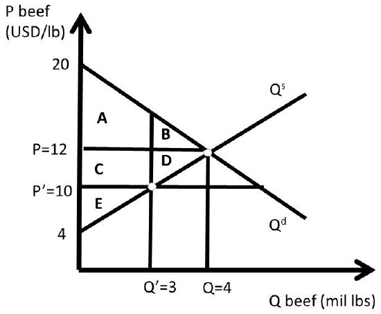
These values, together with the supply and demand functions, allow us to measure the well-being of both consumers and producers before and after the price ceiling policy is implemented (Figure \(\PageIndex{3}\)).

Figure \(\PageIndex{3}\): A Quantitative Price Ceiling in the Beef Market

The free-market equilibrium levels of CS and PS are designated with the subscript 0, calculated in equations \ref{2.3} and \ref{2.4}.

\[CS_0 = A + B = 0.5(20 – 12)(4) = 0.5(8)(4) = \text{ USD } 16 \text{ million} \label{2.3}\]

\[PS_0 = C + D + E = 0.5(12 – 4)(4) = 0.5(8)(4) = \text{ USD } 16 \text{ million} \label{2.4}\]

The level of social welfare is the sum of all surplus in the market, as in Equation \ref{2.5}.

\[SW_0 = A + B + C + D + E = 0.5(20 – 4)(4) = 0.5(16)(4) = \text{ USD } 32 \text{ million} \label{2.5}\]

Assume that the price ceiling is set by the Government at \(P’ = 10\) USD/lb beef. The quantity is found by finding the minimum of quantity supplied and quantity demanded. In the case of a binding price ceiling \((P’ < P)\), the quantity supplied will be the relevant quantity, since producers will produce only \(Q’\) lbs of beef. Consumers will desire to purchase a much larger amount at \(P’ < P\), but are unable to at the lower price \(P’\), since production falls from \(Q\) to \(Q’\). The quantity of \(Q’\) is found by substituting the new price into the inverse supply equation.

\[P = 4 + 2Q^s = 10 = 4 + 2Q^s,\nonumber\]

therefore,

\[Q’ = 3\nonumber\]

The price ceiling \((P’)\) and reduced quantity \((Q’)\) can be seen in Figure \(\PageIndex{3}\). Next, the levels of \(CS, PS,\) and \(SW\)are calculated at the price ceiling level. To find the surplus level of area \(A\), split the shape into one triangle and one rectangle by substitution of \(Q’ = 3\) into the inverse demand curve to get \(P = 14\). Area \(A\) is equal to:\( 0.5(20 – 14)3 + (14 – 12)3 = 9 + 6 = 15\) million USD. We are now ready to calculate the level of surplus for the price ceiling.

\[\begin{align} CS_1 &= A + C = 15 + (12 – 10)(3) = 15 + 6 = \text{ USD 21 million}\\ PS_1 &= E = 0.5(10 – 4)(3) = 0.5(6)(3) = \text{ USD }9 \text{ million}\\SW_1 &= A + C + E = 21 + 9 = \text{ USD 30 million}\end{align}\]

The changes in welfare due to the price ceiling are:

\[\begin{align} ΔCS &= CS_1 – CS_0 = + C – B = 21 – 16 = \text{ USD }+ 5 \text{ million}\\ΔPS &= PS_1 – PS_0 = – C – D = 9 – 16 = \text{ USD }– 7 \text{ million}\\ΔSW &= SW_1 – SW_0 = – B – D = 30 – 32 = \text{ USD } – 2 \text{ million}\end{align}\]

The Dead Weight Loss (DWL) of the price ceiling is the loss to social welfare, of the negative of the change in social welfare:

\[DWL = – ΔSW = 2 \text{ USD million.}\label{2.13}\]

The quantitative analysis of a price ceiling provides timely, important, and interesting results. First, only a subset of consumers are made better off due to a price ceiling. These consumers win because they pay a lower price for the good under the price ceiling than in the free market \((P’ < P)\). Second, some consumers are made worse off due to the price ceiling, since the quantity of the good available is reduced \((Q’ < Q)\). This is because producers reduce the quantity supplied if the price is lowered (the Law of Supply). Third, all producers of the good are made unambiguously worse off due to the price ceiling, since both price and quantity are reduced \((P’ < P; Q’ < Q)\).

The magnitude of the consumer gains and losses are determined by the elasticities of supply and demand. Elastic demand and inelastic supply provide larger consumer benefits, since area \(B\) in Figure \(\PageIndex{3}\) is relatively small under these conditions. If demand is inelastic and supply is elastic, consumers are less likely to gain from the price ceiling, as area \(C\) in Figure \(\PageIndex{3}\) is relatively small in this case.