2.2: Price Support

This section continues the welfare analysis of price policies by investigating the welfare analysis of a price support, also called a minimum price. Price supports are intended to help producers. The outcome of the welfare analysis demonstrates that price supports can increase producer surplus, but in many cases at a large cost to the rest of society. Figure \(\PageIndex{1}\) shows the impact of a price support in the wheat market. This policy is more likely to be enacted in a high-income nation where agricultural producers are a small group that can be more easily subsidized by a large economy.

Price Support = A minimum price policy enacted to help producers.

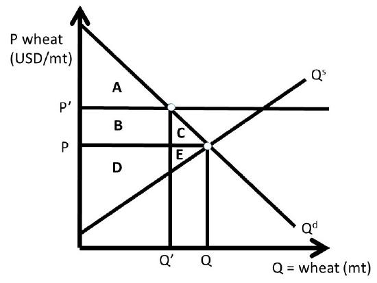
Figure \(\PageIndex{1}\): Case One: Price Support in Wheat Market, No Surplus

The price support mandates that all wheat be bought or sold at a minimum price of \(P^{\prime}\). If the price support were set at a level lower than the market equilibrium price \((P^{\prime} < P)\), it would have no effect (it would not be “binding”). The quantity of wheat on the market depends on how the policy works. There are three possibilities for how the price support is implemented: (1) no surplus exists, (2) the surplus exists, and (3) the government purchases the surplus. Each case will be described in detail in what follows.

Case One: Price Support with No Surplus

The first case is the simplest, but least realistic. In Case One, we assume that producers correctly forecast the quantity demanded, and produce only enough to meet demand. No surplus exists. In Figure \(\PageIndex{1}\), the price support is set by the government at \(P^{\prime}\). It is assumed in this case that producers forego increasing quantity supplied along the supply curve to price \(P^{\prime}\), and instead produce only enough wheat to meet consumer needs, \(Q^{\prime}\):

\[Q^{\prime} = \min(Q^s, Q^d).\nonumber\]

In Case One, no surplus exists. The producers produce and sell only enough wheat to meet the low level of quantity demanded, \(Q^{\prime}\). The initial, free market surplus levels are:

\[\begin{align*} CS_0 &= A + B + C\\ PS_0 &= D + E\\ SW_0 &= A + B + C + D + E \end{align*}\]

After the price support is put in place, the new levels of surplus are;

\[CS_1 = A,\nonumber\]

\[PS_1= B + D,\nonumber\]

and

\[SW_1 = A + B + D.\nonumber\]

Changes in surplus from free markets to the price support with no surplus are:

\[ΔCS = - B - C,\nonumber\]

\[ΔPS = + B - E,\nonumber\]

\[ΔSW = - C - E\nonumber\]

and

\[DWL = -ΔSW = C + E\nonumber\]

Consumers are unambiguously worse off: price is higher \((P^{\prime} > P)\) and quantity is lower \((Q^{\prime} < Q)\), relative to the free market case. Producers may or may not be better off, depending on the relative size of areas B and E. If demand is inelastic and supply is elastic, it is more likely that producer surplus is higher with the price support \((B > E)\). This reflects the analysis of price support in the previous chapter. The producers with low production costs, located on the supply curve between the origin (0, 0) and \(Q^{\prime}\), are made better off since they receive a higher price for the wheat that they produce \((P^{\prime} > P)\). The high-cost producers, located on the supply curve between \(Q^{\prime}\) and \(Q\), are made worse off, since they no longer produce wheat.

The deadweight loss (DWL) equals welfare triangle CE. The price support helps producers, if demand is sufficiently inelastic, but at the expense of the rest of society. In high-income nations such as the US, this policy transfers surplus from the average consumer to producers. Wheat producers have higher levels of income and wealth than the average consumers, so the policy represents a transfer of income to individuals who are better off than the consumers.

Case Two: Price Support When Surplus Exists

Case Two is more realistic than Case One. In Case Two, wheat producers increase quantity supplied to \(Q^{\prime\prime}\), found at the intersection of \(P^{\prime}\) and the supply curve. This is shown in Figure \(\PageIndex{2}\). At the price support level \(P^{\prime}\), consumers purchase only \(Q^{\prime}\), so a surplus exists equal to \(Q^{\prime\prime} – Q^{\prime}\).

Surplus = Quantity supplied minus quantity demanded = \(Q^s – Q^d\).

Note that this surplus of quantity shared the same world as consumer surplus and producer surplus, but refers to an excess quantity instead of an excess value. The initial values of surplus at free market levels are:

\[CS_0 = A + B + C,\nonumber\]

\[PS_0= D + E,\nonumber\]

and

\[SW_0 = A + B + C + D + E.\nonumber\]

After the price support is put in place, the new levels of surplus reflect the large costs of producing the surplus, with no buyers at the high price \((P’ > P)\). The cost of producing the surplus is the area under the supply curve, between \(Q’\) and \(Q’’\): GHI. The area GHI is the cost of producing the surplus, \(Q’’ – Q’\), because it is the area under the supply curve. The surplus levels with the price support, assuming that the surplus exists are:

\[CS_1 = A,\nonumber\]

\[PS_1= B + D – G – H – I,\nonumber\]

and

\[SW_1 = A + B + D – G – H – I.\nonumber\]

Changes in surplus from free markets to the price support with the surplus are:

\[ΔCS = - B - C,\nonumber\]

\[ΔPS = + B - E - G - H - I,\nonumber\]

\[ΔSW = - C - E - G - H - I,\nonumber\]

and

\[DWL = - ΔSW = C + E + G + H + I.\nonumber\]

The impact on consumers remains the same as in Case One, but the impact on producers is much costlier. The surplus is costly to produce, and does not have a buyer. If this policy were to be implemented, the government would have to do something with the surplus of wheat created by the policy, or market forces would put pressure on the wheat market to return to equilibrium.

If the surplus remained, market forces would put downward pressure on the price of what making the price support more difficult and more expensive to maintain. This leads to Case Three, where the government purchases the surplus grain and removes it from the market, described in the next section.

Figure \(\PageIndex{2}\): Case Two: Price Support in Wheat Market, Surplus Exists

Case Three: Price Support When Government Purchases Surplus

The surplus created by a price support is costly to producers, and if nothing is done to eliminate the surplus, the policy does not achieve the objective of helping producers. There are three methods for the government to eliminate the surplus:

1. Destroy the surplus,
2. Give the surplus away domestically, or
3. Give the surplus away internationally.

In all three cases, the government purchases the surplus at the price support level. This is the only way to maintain the price support. Without government purchases, the surplus would result in market forces that put downward pressure on the price of wheat. Destroying the surplus is not politically popular, since it involves eliminating food when there are hungry people in the world. The US did this in earlier decades by dumping surplus grain in the ocean, killing baby pigs, and dumping milk on the ground. This was not popular with consumers, producers, or politicians. The practice of destroying food to maintain higher food prices is not used today.

Domestic food programs make more sense as a method for eliminating the surplus. School breakfast and school lunch programs make use of the food surpluses by assisting those in need. Food aid is using the surplus food from the USA to alleviate hunger in other nations. Food aid and other forms of international assistance are popular programs that help the US producers and the recipient nation’s consumers. Food aid can be controversial, since it lowers food prices in receiving nations, and can cause “dependency” of the recipient on the donor nation.

Food aid results in lower prices, which cause a decrease in the quantity of food supplied in the recipient nation. Although food aid may alleviate hunger and/or starvation, it decreases the incentives for a nation to produce food. This is a true paradox, making food and agricultural policy a challenge for policy makers: there are winner and losers that result from all public policies.

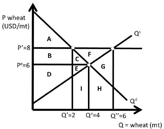
Case Three is shown in Figure \(\PageIndex{3}\), where the government purchases the surplus \((Q’’ – Q’)\).

As in the two previous cases, the initial values of surplus at free market levels are:

\[CS_0 = A + B + C,\nonumber\]

\[PS_0= D + E,\nonumber\]

\[G_0 = 0,\nonumber\]

and

\[SW_0 = A + B + C + D + E.\nonumber\]

Note that the government \((G)\) is included in this case of the price support. After the price support is put in place, the new levels of surplus reflect the large costs of the government buying the surplus. The cost of producing the surplus \((Q’’ – Q’)\) at the price support level equals \(P’\) multiplied by \((Q’’ – Q’)\), which is equal to area \(CEFGHI\) (Figure \(\PageIndex{3}\)), the cost of producing the surplus. The surplus levels with the price support, assuming that the surplus exists are:

\[CS_1 = A,\nonumber\]

\[PS_1= B + C + D + E + F,\nonumber\]

\[G_1 = – C – E – F – G – H – I,\nonumber\]

and

\[SW_1 = A + B + D – G – H – I.\nonumber\]

Changes in surplus from free markets to the price support with the surplus are:

\[ΔCS = - B - C,\nonumber\]

\[ΔPS = + B + C + F,\nonumber\]

\[ΔG = - C - E - F - G - H - I,\nonumber\]

\[ΔSW = - C - E - G - H - I,\nonumber\]

and

\[DWL = - ΔSW = C + E + G + H + I.\nonumber\]

Figure \(\PageIndex{3}\): Case Three: Price Support in Wheat Market, Government Purchases Surplus

The total societal surplus changes are identical in Cases Two and Three: \(DWL = CEGHI\) in both cases. The distribution of benefits is quite different, however. In Case Two, the producers bear the large costs of overproduction: \(-GHI\). In Case Two, the government has attempted to help producers, but has decreased producer surplus due to the unintended consequence of wheat growers producing too much food at the high level of the price support. If the government does purchase the surplus as in Case 3, these high costs are shifted to taxpayers, and producers are helped by the price support program.

The price support does meet the objective of helping producers in Case 3, but at a high cost to society. As in the case of the price ceiling, the price support results in losses to society \((DWL > 0)\). This is true of all government interventions into the market. The maximum level of surplus occurs with free markets and free trade. In food and agriculture, there are numerous cases of government intervention into markets, reflecting objectives other than maximizing social welfare.

In some circumstances, policy makers determine that the distributional consequences of a policy are more important than maximizing social welfare. In these cases, who gets what determines policy outcomes, rather than the overall efficiency of the market.

Quantitative Analysis of a Price Support

In this example, wheat producers are successful in their efforts to convince Congress to pass a law that authorizes a price support for wheat. Suppose that the inverse supply and demand for wheat are given by:

\[P = 10 – Q^d, \label{2.1}\]

and

\[P = 2 + Q^s.\label{2.2}\]

Where \(P\) is the price of wheat in USD/MT, and \(Q\) is the quantity of wheat in million metric tons (MMT). The equilibrium price \((P^e)\) and quantity of wheat \((Q^e)\)are calculated by setting the inverse supply and demand equations equal to each other to achieve:

\[P^e = \text{USD } 6\text{/MT wheat,}\nonumber\]

and

\[Q^e = 4 \text{ MMT wheat.}\nonumber\]

These values, together with the supply and demand functions, allow us to measure the changes in surpluses for both consumers and producers due to the price support (Figure \(\PageIndex{4}\)).

Figure \(\PageIndex{4}\): Case One: Quantitative Price Support in Wheat Market, No Surplus

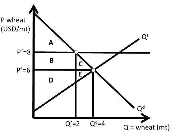
The calculations will proceed by directly determining the changes in surplus, rather than calculating the initial and ending values of surplus, as we did above for the price ceiling. To find the dollar values of the areas in Figure \(\PageIndex{4}\), recall that you can always find a price or quantity by substitution of a \(P\) or \(Q\) into the inverse supply or inverse demand curve. There is always enough information provided to find prices, quantities, and the areas that represent surplus values.

Assume that the price support is set at \(P’ = 8\) USD/MT wheat. The quantity is found by the minimum of quantity demanded \((Q^d)\) and quantity supplied \((Q^s)\): \(\min(Q^s, Q^d)\). Therefore, the quantity is \(Q’ = Q^d\), the quantity demanded. Surplus changes are:

\[\begin{align*} ΔCS &= – B – C = – 4 – 2 = – 6 \text{ USD million} \\[4pt] ΔPS &= + B – E = + 4 – 2 = + 2 \text{ USD million} \\[4pt] ΔG &= 0\\[4pt] ΔSW &= – C – E = – 2 – 2 = – 4 \text{ USD million}\\ DWL &= – ΔSW = C + E = + 4 \text{ USD million} \end{align*}\]

The government does nothing in Case One, and wheat producers supply only enough wheat to the market to meet consumer demand. Case Two is shown in Figure \(\PageIndex{5}\). In Case Two, producers produce a large amount of wheat \((Q’’)\) due to the high price \(P’\). There is a large surplus created, but in this case there is no intervention by the government. Wheat producers have very large costs, since they produce 6 million metric tons \((Q’’)\), and consumers only purchase 2 million metric tons (\(Q’\), Figure \(\PageIndex{5}\)).

Figure \(\PageIndex{5}\): Case Two: Quantitative Price Support in Wheat Market, Surplus Exists

\[\begin{align*} ΔCS &= – B – C = – 4 – 2 = – 6 \text{ USD million}\\ΔPS &= + B – E – G – H – I = + 4 – 26 = – 22 \text{ USD million}\\ΔG &= 0\\ΔSW &= – C – E – G – H – I = – 28 \text{ USD million}\\DWL &= – ΔSW = C + E + G + H + I = + 28 \text{ USD million}\end{align*}\]

In Case Three, the government intervenes and buys the surplus. This allows the price to stay at the price support level, \(P’\). Quantity supplied and quantity demanded are at the same levels as in Case Two, but the government’s expenses are large, and wheat producers benefit from the high price \((P’ > P^e)\) and larger quantity sold \((Q’’ > Q^e\), Figure \(\PageIndex{6}\)).

Figure \(\PageIndex{6}\): Case Three: Quantitative Wheat Price Support, Government Buys Surplus

\[\begin{align*} ΔCS &= – B – C = – 4 – 2 = – 6 \text{ USD million}\\ΔPS &= + B + C + F = 4 + 2 + 4 = + 10 \text{ USD million}\\ΔG &= – C – E – F – G – H – I = – 32 \text{ USD million}\\ΔSW &= – C – E – G – H – I = – 28 \text{ USD million}\\DWL &= – ΔSW = C + E + G + H + I = + 28 \text{ USD million}\end{align*}\]

In Case Three, the price support has large costs, paid for by the government. One benefit that is not explicitly included is the food aid that could be provided to domestic and foreign consumers. These benefits would provide noneconomic gains, but no added surplus value to the program. Price supports can increase producer surplus, but at a cost. Government interventions often have unintended consequences, such as the surplus of grain in this case.

After World War II, European nations subsidized food and agriculture heavily. Since they had experienced massive food shortages during the War, Europeans did not want to rely on other nations for food. The large subsidies resulted in large surpluses of food that had to be exported at below-market prices to maintain the high food prices within Europe. In the next section, we will discuss quantitative restrictions as another means of increasing prices in food and agriculture.