
2.4: Import Quota
- Last updated
- Save as PDF
- Page ID
- 43154

The large benefits of free trade have been emphasized in this book. Free markets and free trade are based on voluntary, mutually-beneficial transactions that make both trading partners better off. The global economic gains from free trade have been enormous, as they enhance efficiency of resource use. Comparative advantage and gains from trade allow each individual, firm, or nation to “do what they do best, and trade for the rest.”
Not everyone wins from trade, however. As was emphasized in Section 1.6.3 above, the overall net benefits are positive, but there are winners and losers from trade. Specifically, producers in importing nations and consumers in exporting nations lose due to price changes that negatively affect them. Like all public policies, free trade has winners and losers. The overall size of the economy is maximized under free markets and free trade, but there are distributional consequences that result in winners and losers.
Trade barriers are most often erected to protect domestic producers from imports. Sugar is produced in the United States, but at higher production costs than sugar production in tropical climates found in Cuba, the Dominican Republic, and Haiti. If free trade prevailed, all sugar consumed in the USA would be imported, since it is cheaper to buy sugar than to produce it domestically. Sugar producers are interested in maintaining sugar production in the USA, as this is how they make their living. Agricultural trade policy has limited sugar imports to a much smaller amount than the free trade level, through a sugar quota, demonstrated in Figure \(\PageIndex{1}\). The import reduction makes sugar in the USA more scarce, and therefore more valuable.
In a closed economy, market forces ensure that supply and demand are equal \((Q^s = Q^d)\). If the USA were a closed economy, the price of sugar would be very high, well above the world market price of sugar \(P_w\). Suppose that the USA is a “small nation” purchaser of sugar: this means that the USA is a “price taker,” facing a constant world price of sugar for all quantities purchased. The assumption of an importing nation being a small nation, or price taker, simplifies our analysis. In the real world, the importer may be large enough to influence the world price of sugar through large purchases of sugar on the global market.
This is represented as a horizontal line at Pw in Figure \(\PageIndex{1}\). At the world price of \(P_w\), the USA would produce \(Q^s\) domestically and consume \(Q^d\). The difference between quantity demanded and quantity supplied is imports \((Q^d – Q^s)\). The equality of domestic supply and demand has been broken by the ability to import less expensive sugar from other nations. Note that in a situation with no imports, the domestic price in the USA would be at the intersection of \(Q^s\) and \(Q^d\).
Domestic sugar producers lobby the government for protection, and receive it in the form of a sugar quota, meaning a maximum amount of sugar imports. The right to import sugar is auctioned off to the highest bidders, who pay for the right to import sugar. Suppose that the quota is set at \(Q^{d’} – Q^{s’}\). This level of quota is binding, since \((Q^{d’} – Q^{s’}) < (Q^d – Q^s)\).

This level of imports is the horizontal distance between \(Q^{d’}\) and \(Q^{s’}\) in Figure \(\PageIndex{1}\). At this quota level, the price of sugar increases to \(P’\), since the quantity of sugar in the market is reduced from free market levels. At this high price \((P’ > P_w)\), quantity supplied increases from \(Q^s\) to \(Q^{s’}\), and quantity demanded decreases from \(Q^d\) to \(Q^{d’}\). These changes are due to the quota, which decreases the amount of sugar allowed into the country. Sugar producers are pleased with this policy, since the price is higher and domestic quantity supplied \((Q^{s’} > Q^s)\) larger.
Welfare Analysis of an Import Quota
The welfare analysis of the import quota identifies the changes in economic surplus of producers, consumers, and the government. The government gains from selling the import quota permits to the sugar importers. These firms will compete with each other to win the right to import sugar. The firms will bid up the price in an auction until the price is equal to the market value of the quota. In this case, the market value is equal to \((P’ – P_w)\), since this is the gain from importing one pound of sugar into the USA. The complete welfare analysis is:
\[ΔCS = – A – B – C – D,\nonumber\]
\[ΔPS = + A,\nonumber\]
\[ΔG = + C,\nonumber\]
\[ΔSW = – B – D,\nonumber\]
and
\[DWL = B + D.\nonumber\]
Producers gain, but with large costs to consumers. The government gains from the sale of the quota permits (or licenses) to sugar importers. Sugar consumers are made much worse off from this policy. The area \(B\) is called the “production loss” of the policy. This area is equal to the losses of using scarce resources to produce sugar in the USA instead of buying it at the world price. Area \(B\) represents the production costs, since it is the area under the supply curve, and above the world price \((P_w)\). These resources could be more efficiently used producing something other than sugar. Area \(D\) is called the “consumption loss” of the import quota. This is the area under the demand curve and above the world price \((P_w)\), which represents the extra dollars spent by US consumers buying domestic sugar instead of low-cost imported sugar. Areas \(B\) and \(D\) represent the loss in social welfare, or the deadweight loss, of the government intervention. Free markets and free trade would provide efficiency of resource use and lower costs to consumers.
In the USA, sugar prices are typically one to two times higher than the world price, resulting in billions of dollar losses to sugar consumers. This policy also has an interesting unintended consequence. High fructose corn syrup (HFCS) is a perfect substitute in consumption for sucrose (sugar made from sugar cane or sugar beets). Corn producers lobby the government to maintain the sugar import quota, to keep the price of sugar high. When the sugar price is high, buyers of sugar (Coca Cola, Pepsi, Mars, etc.) switch out of sucrose and into fructose. Corn farmers are among the largest supporters of the sugar import quota! The positive impact on corn producers is a truly unique and unanticipated cause and effect of protection of domestic sweetener producers from foreign competition.
Quantitative Welfare Analysis of an Import Quota
Suppose that the inverse demand and supply of sugar are given by:
\[P = 100 – Q^d,\nonumber\]
and
\[P = 10 + Q^s,\nonumber\]
Where \(P\) is the price of sugar in USD/lb, and \(Q\) is the quantity of sugar in million pounds. Suppose also that the world price of sugar is given by \(P_w = 20\) USD/lb, as shown in Figure \(\PageIndex{2}\). In a closed economy, there would be no imports or exports, so \(Q^s = Q^d\) at this market equilibrium, where supply is equal to demand:
\[Q^e = 45 \text{ million pounds of sugar}\nonumber\]
and
\[P^e = 55 \text{ USD/lb}.\nonumber\]
This is a high price of sugar relative to the world price, occurring at the intersection of \(Q^s\) and \(Q^d\) in Figure \(\PageIndex{2}\). If imports are allowed, the USA can break the equality of production and consumption \((Q^s \neq Q^d)\) through imports of less expensive sugar \((Q^s < Q^d)\). If we assume that the USA is a “small nation” in sugar trade, then the USA is a price taker, and can import as much or as little sugar as it desires at the world price. Note that a “large nation” means that a country is a price maker, and has enough market power to influence the price of the imported good.
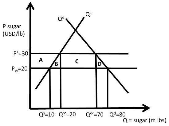
The free market equilibrium in an open economy can be calculated by substitution of the world price into the inverse supply and demand functions. At the world price, \(Q^s = 10\) m lbs sugar and \(Q^d = 80\) m lbs sugar. Imports are equal to \(Q^s – Q^d = 70\) m lbs sugar. Social welfare is maximized at this free trade equilibrium, since sugar is produced by the lowest cost producers. Ten million pounds of sugar are produced by domestic producers along the supply curve below the world price, and 70 m lbs are produced by foreign sugar producers at the world price of 20 USD/lb.
Now assume that a sugar import quota is implemented, equal to 50 m lbs of sugar. To be binding, the import quota must be less than the free-market level of imports. Since this is less than the free trade import level, it will decrease the amount of sugar available in the USA, and cause price to increase. The sugar price that results from the quota \((P’)\) can be calculated using the inverse supply and demand curves and the import quota:
\[Q^{d’} – Q^{s’} = 50,\nonumber\]
\[P’ = 100 – Q^{d’},\nonumber\]
and
\[P’ = 10 + Q^{s’}.\nonumber\]
Rearranging the first equation: \(Q^d = 50 + Q^s\). Substitution of the first equation into the inverse demand equation yields:
\[P’ = 100 – (50 + Q^{s’}) = 50 – Q^{s’}.\nonumber\]
This equation can be set equal to the inverse supply equation:
\[P’ = 50 – Q^{s’} = 10 + Q^{s’}.\nonumber\]
Solving for \(Q^{s’}\):
\[2Q^{s’} = 50 – 10,\nonumber\]
or
\[Q^{s’} = 40/2 = 20 \text{ m lbs sugar}.\nonumber\]
Substituting this into the import equation and the inverse supply function yield:
\[P’ = 30 \text{ USD/ lb},\nonumber\]
and
\[Q^{d’} = 70 \text{ m lbs sugar}.\nonumber\]
These values are all shown in Figure \(\PageIndex{2}\). Notice that quantity supplied has increased \((Q^{s’} > Q^s)\) and quantity demanded has decreased \((Q^{d’} < Q^d)\) due to the import quota and the resulting higher price \((P’ > P_w)\). The welfare analysis can now be conducted by calculation of the areas in the graph.
\[\begin{align*} ΔCS &= – A – B – C – D = – 750 \text{ USD million}\\ ΔPS &= + A = + 150 \text{ USD million}\\ΔG &= + C = + 500 \text{ million}\\ΔSW &= – B – D = – 100 \text{ USD million}\\ DWL &= B + D = + 100 \text{ million}\end{align*}\]
The government gains area \(C\) by auctioning off the permits that allow firms to import sugar. The quantitative results confirm that import restrictions help domestic producers, but at thigh costs to domestic consumers. The high price for sugar also provides support to corn producers, since High Fructose Corn Syrup (HFCS) is a close substitute to sucrose. Taxes are analyzed in the next section.