We have located the profit-maximizing level of output and price for a monopoly. How does the monopolist know that this is the correct level? How is the profit-maximizing level of output related to the price charged, and the price elasticity of demand? This section will answer these questions. The firm’s own price elasticity of demand captures how consumers of a good respond to a change in price. Therefore, the own price elasticity of demand captures the most important thing that a firm can know about its customers: how consumers will react if the good’s price is changed.
The Monopolist’s Tradeoff between Price and Quantity
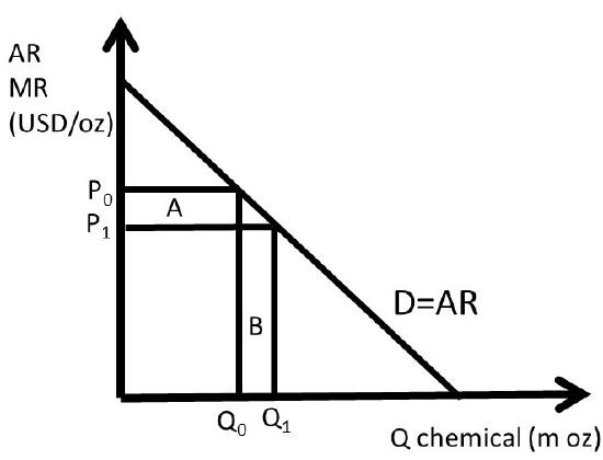
What happens to revenues when output is increased by one unit? The answer to this question reveals useful information about the nature of the pricing decision for firms with market power, or a downward sloping demand curve. Consider what happens when output is increased by one unit in Figure \(\PageIndex{1}\).
Figure \(\PageIndex{1}\): Per-Unit Revenues for a Monopolist: Agricultural Chemical
Increasing output by one unit from \(Q_0\) to \(Q_1\) has two effects on revenues: the monopolist gains area \(B\), but loses area \(A\). The monopolist can set price or quantity, but not both. If the output level is increased, consumers’ willingness to pay decreases, as the good becomes more available (less scarce). If quantity increases, price falls. The benefit of increasing output is equal to \(ΔQ\cdot P_1\), since the firm sells one additional unit \((ΔQ)\) at the price \(P_1\) (area \(B\)). The cost associated with increasing output by one unit is equal to \(ΔP\cdot Q_0\), since the price decreases \((ΔP)\) for all units sold (area \(A\)). The monopoly cannot increase quantity without causing the price to fall for all units sold. If the benefits outweigh the costs, the monopolist should increase output: if \(ΔQ\cdot P_1 > ΔP\cdot Q_0\), increase output. Conversely, if increasing output lowers revenues \((ΔQ\cdot P_1 < ΔP\cdot Q_0)\), then the firm should reduce output level.
The Relationship between MR and Ed
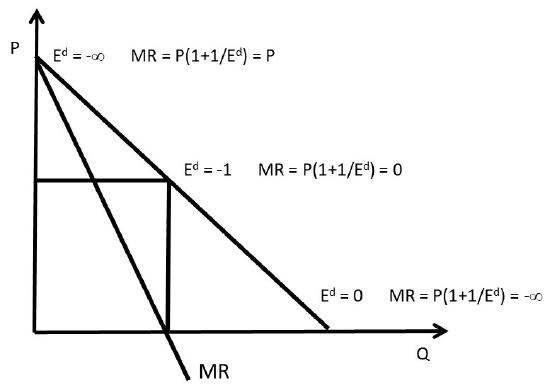
There is a useful relationship between marginal revenue \((MR)\) and the price elasticity of demand \((E^d)\). It is derived by taking the first derivative of the total revenue \((TR)\) function. The product rule from calculus is used. The product rule states that the derivative of an equation with two functions is equal to the derivative of the first function times the second, plus the derivative of the second function times the first function, as in Equation \ref{3.3}.
The product rule is used to find the derivative of the \(TR\) function. Price is a function of quantity for a firm with market power. Recall that \(MR = \frac{∂TR}{∂Q}\), and the equation for the elasticity of demand:
This is a useful equation for a monopoly, as it links the price elasticity of demand with the price that maximizes profits. The relationship can be seen in Figure \(\PageIndex{2}\).
Figure \(\PageIndex{2}\): The Relationship between MR and Ed
At the vertical intercept, the elasticity of demand is equal to negative infinity (section 1.4.8). When this elasticity is substituted into the \(MR\) equation, the result is \(MR = P\). The \(MR\) curve is equal to the demand curve at the vertical intercept. At the horizontal intercept, the price elasticity of demand is equal to zero (Section 1.4.8, resulting in \(MR\) equal to negative infinity. If the \(MR\) curve were extended to the right, it would approach minus infinity as \(Q\) approached the horizontal intercept. At the midpoint of the demand curve, \(P\) is equal to \(Q\), the price elasticity of demand is equal to \(-1\), and \(MR = 0\). The \(MR\) curve intersects the horizontal axis at the midpoint between the origin and the horizontal intercept.
This highlights the usefulness of knowing the elasticity of demand. The monopolist will want to be on the elastic portion of the demand curve, to the left of the midpoint, where marginal revenues are positive. The monopolist will avoid the inelastic portion of the demand curve by decreasing output until \(MR\) is positive. Intuitively, decreasing output makes the good more scarce, thereby increasing consumer willingness to pay for the good.
Pricing Rule I
The useful relationship between \(MR\) and \(E_d\) in Equation \ref{3.4} can be used to derive a pricing rule.
\[\begin{align*} MC &= P + \frac{P}{E_d}\\[4pt] –\frac{P}{E_d} &= P – MC\\[4pt] –\frac{1}{E_d} &= \frac{P – MC}{P}\\[4pt] \frac{P – MC}{P} &= –\frac{1}{E_d}\end{align*}\]
This pricing rule relates the price markup over the cost of production \((P – MC)\) to the price elasticity of demand.
\[\frac{P – MC}{P} = –\frac{1}{E_d} \label{3.5}\]
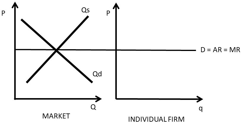
A competitive firm is a price taker, as shown in Figure \(\PageIndex{3}\). The market for a good is depicted on the left hand side of Figure \(\PageIndex{3}\), and the individual competitive firm is found on the right hand side. The market price is found at the market equilibrium (left panel), where market demand equals market supply. For the individual competitive firm, price is fixed and given at the market level (right panel). Therefore, the demand curve facing the competitive firm is perfectly horizontal (elastic), as shown in Figure \(\PageIndex{3}\).
The price is fixed and given, no matter what quantity the firm sells. The price elasticity of demand for a competitive firm is equal to negative infinity: \(E_d = -\inf\). When substituted into Equation \ref{3.5}, this yields \((P – MC)P = 0\), since dividing by infinity equals zero. This demonstrates that a competitive firm cannot increase price above the cost of production: \(P = MC\). If a competitive firm increases price, it loses all customers: they have perfect substitutes available from numerous other firms.
Monopoly power, also called market power, is the ability to set price. Firms with market power face a downward sloping demand curve. Assume that a monopolist has a demand curve with the price elasticity of demand equal to negative two: \(E_d = -2\). When this is substituted into Equation \ref{3.5}, the result is: \(\dfrac{P – MC}{P} = 0.5\). Multiply both sides of this equation by price \((P)\): \((P – MC) = 0.5P\), or \(0.5P = MC\), which yields: \(P = 2MC\). The markup (the level of price above marginal cost) for this firm is two times the cost of production. The size of the optimal, profit-maximizing markup is dictated by the elasticity of demand. Firms with responsive consumers, or elastic demands, will not want to charge a large markup. Firms with inelastic demands are able to charge a higher markup, as their consumers are less responsive to price changes.
Figure \(\PageIndex{3}\): The Demand Curve of a Competitive Firm
In the next section, we will discuss several important features of a monopolist, including the absence of a supply curve, the effect of a tax on monopoly price, and a multiplant monopolist.